library(ggplot2)
library(patchwork)

te_paper  <- "#f5f4ee"
te_ink    <- "#16241d"
te_body   <- "#2c3a31"
te_forest <- "#275139"
te_rust   <- "#b5534e"
te_gold   <- "#c9b458"
te_line   <- "#dad9ca"

theme_datasheet <- function() {
  theme_minimal(base_size = 12) +
    theme(plot.background  = element_rect(fill = te_paper, colour = NA),
          panel.background = element_rect(fill = te_paper, colour = NA),
          panel.grid.major = element_line(colour = te_line, linewidth = 0.3),
          panel.grid.minor = element_blank(),
          text             = element_text(colour = te_body),
          plot.title       = element_text(colour = te_ink, face = "bold"),
          plot.subtitle    = element_text(colour = te_body),
          axis.text        = element_text(colour = te_body))
}Levy walk or patchy habitat: which test to trust
R
movement ecology
Levy walk
power law
simulation
ecology tutorial
A Brownian walker whose speed changes with habitat can pass the power-law tail test for a Levy walk. In R: which protocols it fools, and the serial check.
A GPS collar on a foraging seal, or a tag on a wandering albatross, returns a few thousand displacements between fixes. Most are short, a handful are enormous, and on a log-log plot of the share of steps longer than a given length the upper end runs close to a straight line. The next sentence of many papers written in the Levy-flight years was that the animal performs a Levy walk: a search strategy with step lengths drawn from a power law, with an exponent near two that theory calls optimal for sparse, randomly placed prey. The claim is about the animal’s rule. The data are a list of step lengths.
The trouble is old and has names. Benhamou showed in 2007 that a composite walk, an animal that switches between a slow intensive search and a fast extensive one, each with ordinary short-tailed steps, produces step length distributions that pass for power laws. Petrovskii, Mashanova and Jansen showed in 2011 that individuals which each move with exponential steps, but at different speeds, pool into a heavy-tailed distribution that looks like a Levy flight, and Jansen and the same colleagues showed in a 2012 comment that a Levy walk reported in mussels was better described by a composite Brownian walk once more candidate models were compared. Edwards and colleagues had already revisited the albatross, bumblebee and deer data behind the first Levy flight claims and found that the power law did not survive once the data were refitted by likelihood. This post is a demonstration of those published results, not a claim to them. What it measures is narrower: how often each common protocol calls a Brownian walker a Levy walker, across kinds of habitat heterogeneity and two track lengths, and in which order the checks should be run.
The neighbours on this site come at pieces of the problem from other sides. When a mixture is really skewness shows a two-component mixture wrongly beating a single skewed law, and repairs it with a second measurement. Here the error runs the other way: a single heavy-tailed law beats a truth that is a mixture of a few speeds, and whether it wins depends mostly on which test is run. A tail-only comparison against one exponential, the comparison most likely to produce a Levy verdict, gives the power law a single rival that cannot represent a mixture at all. Fitting a body size spectrum uses the same Kolmogorov-Smirnov scan over a lower limit that the tail test below uses, and its warning that the lower limit “is the one that moves the answer furthest” applies here too, but it has no movement and no mixture alternative. Step lengths and turning angles in R fits gamma and Weibull laws to one correlated random walk by maximum likelihood and AIC, with no heavy tail in sight.
The last check in the post is not new either. Checking a movement HMM fits a one-state model to a two-state track in its section on what a wrong model looks like, and finds the marginal passable while the lag-one autocorrelation of the pseudo-residuals gives the wrong model away: “A model that misses the state dynamics leaves the dependence in the residuals even when the marginal shape looks passable.” The serial test used below is that device applied to raw steps, and the link between the two is exact, as the section on order shows.
A walker that is Brownian everywhere
q_switch <- 0.05
min_tail <- 50

gen_track <- function(type, n, q = q_switch, hi = 10, shape = 1.5) {
  if (type == "levy") return((1 - runif(n))^(-1))
  new_patch  <- c(TRUE, runif(n - 1) < q)
  patch_id   <- cumsum(new_patch)
  n_patch    <- patch_id[n]
  patch_mean <- switch(type,
    h2 = sample(c(1, hi), n_patch, replace = TRUE),
    h3 = sample(c(1, 3, 9), n_patch, replace = TRUE),
    ln = exp(rnorm(n_patch, 0, 1)),
    ga = 1 / rgamma(n_patch, shape = shape, rate = shape))
  rexp(n, 1 / patch_mean[patch_id])
}

patches_1000 <- 1 + 999 * q_switch
patches_300  <- 1 + 299 * q_switch

cv_disc <- function(m_vals) sqrt(mean(m_vals^2) - mean(m_vals)^2) / mean(m_vals)
cv_mean <- c(h2_5 = cv_disc(c(1, 5)), h2_10 = cv_disc(c(1, 10)),
             h3 = cv_disc(c(1, 3, 9)), ln = sqrt(exp(1) - 1), ga3 = 1 / sqrt(3 - 2))

cell_tab <- data.frame(
  cell  = c("2 habitats, 1:5", "2 habitats, 1:10", "3 habitats, 1:3:9",
            "lognormal", "gamma, shape 3", "gamma, shape 1.5",
            "iid 2 habitats", "iid gamma 1.5", "Levy, mu 2"),
  type  = c("h2", "h2", "h3", "ln", "ga", "ga", "h2", "ga", "levy"),
  hi    = c(5, 10, NA, NA, NA, NA, 10, NA, NA),
  shape = c(NA, NA, NA, NA, 3, 1.5, NA, 1.5, NA),
  q     = c(rep(q_switch, 6), 1, 1, NA),
  group = c(rep("discrete habitats", 3), rep("continuous speeds", 3),
            rep("controls", 3)))

draw_cell <- function(i, n) {
  arg <- list(type = cell_tab$type[i], n = n)
  if (!is.na(cell_tab$hi[i]))    arg$hi    <- cell_tab$hi[i]
  if (!is.na(cell_tab$shape[i])) arg$shape <- cell_tab$shape[i]
  if (!is.na(cell_tab$q[i]))     arg$q     <- cell_tab$q[i]
  do.call(gen_track, arg)
}
Every non-Levy walker below draws each step from an exponential distribution, so within a habitat it is a plain Brownian walker in the sense of the Levy literature: short tailed, with no memory of step length beyond what the habitat imposes. The habitat is what changes. At each step, with probability 0.05, the walker enters a new patch and a new mean step is drawn; otherwise it stays in the patch it is in. Patches therefore last 20 steps on average, and a 1000-step track visits about 51 patches in expectation, a 300-step track about 16.
The patch means come in six persistent kinds, and the order matters for what follows. Three are discrete: two habitats with mean steps of 1 and 5, two habitats with 1 and 10, and three habitats with 1, 3 and 9, each drawn with equal probability. Three are continuous: a lognormal mean step with a log standard deviation of 1, and a gamma-distributed movement rate, the reciprocal of the mean step, with shape 3 and with shape 1.5. The gamma cells are the heavy end on purpose. If the rate is gamma with shape a and rate a and the step given the rate is exponential, the marginal step length has survival function (1 + x / a) raised to the power minus a, which is a Lomax distribution: its density falls off with a tail exponent of a + 1, so 2.5 at shape 1.5 and 4 at shape 3. A gamma rate builds a power law into the habitat itself: the patch mean steps, the reciprocals of the rate, have a density tail with the same exponent a + 1, and at shape 2 or below their variance is infinite (shape 3 gives a finite one, with a coefficient of variation of 1.00). That is why the gamma cells come after the discrete ones, with shape 1.5 last.
Three controls sit beside them. Two redraw the speed at every step instead of every patch (the iid cells, with q = 1), with two habitats at 1 and 10 and with a gamma rate of shape 1.5; the second of these has an exactly Lomax marginal and no serial structure at all, which gives the same pooled marginal as Petrovskii’s setting, individuals that each keep their own speed. The third is a true Levy walker, independent Pareto steps with tail exponent mu = 2 and a minimum step of 1.
Three protocols and one serial check
The protocols follow the ones argued over in the Levy debate, written out in base R. The power law is fitted by maximum likelihood above a lower limit xmin chosen by the Kolmogorov-Smirnov scan that Clauset, Shalizi and Newman recommend, over the 0 to 90 per cent quantiles of the track in steps of 2 per cent, keeping at least 50 steps above the limit. The exponential alternative on that tail is shifted to start at xmin, so both models are densities on the same range and their AIC values are comparable. The two-exponential mixture is fitted by EM from three starts, on the same shifted tail.
pl_fit <- function(z, xm) {
  s_log <- sum(log(z / xm))
  k     <- length(z)
  mu    <- 1 + k / s_log
  c(ll = k * log(mu - 1) - k * log(xm) - mu * s_log, mu = mu)
}

exp_ll <- function(y) length(y) * (-log(mean(y)) - 1)

mix2_fit <- function(y, n_it = 500, tol = 1e-9) {
  best <- list(ll = -Inf)
  for (s_q in c(0.2, 0.5, 0.8)) {
    m_k <- unname(quantile(y, c(s_q / 2, 0.5 + s_q / 2)))
    w_1 <- 0.5
    ll_old <- -Inf
    for (it in seq_len(n_it)) {
      l_1   <- log(w_1) - log(m_k[1]) - y / m_k[1]
      l_2   <- log(1 - w_1) - log(m_k[2]) - y / m_k[2]
      l_max <- pmax(l_1, l_2)
      l_tot <- l_max + log(exp(l_1 - l_max) + exp(l_2 - l_max))
      ll    <- sum(l_tot)
      if (ll - ll_old < tol * abs(ll)) break
      ll_old <- ll
      g_1 <- exp(l_1 - l_tot)
      w_1 <- mean(g_1)
      if (w_1 < 1e-4 || w_1 > 1 - 1e-4) break
      m_k <- c(sum(g_1 * y) / sum(g_1), sum((1 - g_1) * y) / sum(1 - g_1))
    }
    if (is.finite(ll) && ll > best$ll) best <- list(ll = ll, w = w_1, m = m_k)
  }
  best
}

ks_xmin <- function(x) {
  cand <- unique(unname(quantile(x, seq(0, 0.9, by = 0.02), type = 1)))
  ks_d <- vapply(cand, function(xm) {
    z <- sort(x[x > xm])
    k <- length(z)
    if (k < min_tail) return(Inf)
    mu    <- 1 + k / sum(log(z / xm))
    f_fit <- 1 - (z / xm)^(1 - mu)
    max(pmax(seq_len(k) / k - f_fit, f_fit - (seq_len(k) - 1) / k))
  }, 0)
  cand[which.min(ks_d)]
}

lag1_test <- function(x) {
  n_pair <- length(x) - 1
  r_s <- cor(rank(x[-length(x)]), rank(x[-1]))
  c(rho = r_s,
    p = pt(r_s * sqrt((n_pair - 2) / (1 - r_s^2)), n_pair - 2, lower.tail = FALSE))
}

score_track <- function(x) {
  xm <- ks_xmin(x)
  z  <- x[x > xm]
  y  <- z - xm
  pl <- pl_fit(z, xm)
  aic_tail <- c(pl = 2 - 2 * pl[["ll"]], ex = 2 - 2 * exp_ll(y),
                mx = 6 - 2 * mix2_fit(y)$ll)
  mu_ok <- pl[["mu"]] > 1 && pl[["mu"]] <= 3
  xm_w <- min(x)
  z_w  <- x[x > xm_w]
  y_w  <- z_w - xm_w
  aic_whole <- c(pl = 2 - 2 * pl_fit(z_w, xm_w)[["ll"]], ex = 2 - 2 * exp_ll(y_w),
                 mx = 6 - 2 * mix2_fit(y_w)$ll)
  lag_res <- lag1_test(x)
  c(call_exp = aic_tail[["pl"]] < aic_tail[["ex"]] && mu_ok,
    call_mix = aic_tail[["pl"]] < min(aic_tail[c("ex", "mx")]) && mu_ok,
    whole_pl = unname(which.min(aic_whole)) == 1,
    lag1     = lag_res[["p"]] < 0.05,
    mu = pl[["mu"]], n_tail = length(z), xmin = xm,
    pearson1 = cor(x[-length(x)], x[-1]), rho = lag_res[["rho"]])
}
Protocol 1 calls a track Levy when the power law beats the single exponential by AIC on the tail and the fitted exponent lies in the Levy range, above 1 and at most 3. Protocol 2 is the same call with the two-exponential mixture added as a second alternative, so the power law has to beat both. Protocol 3 ignores xmin and fits all three laws from the smallest step, and asks whether the power law has the lowest AIC. The serial check is a one-sided test of positive lag-one Spearman correlation between successive steps at the 5 per cent level.
set.seed(2711)
repeat {
  x_ex <- draw_cell(2, 1000)
  s_ex <- score_track(x_ex)
  if (s_ex[["call_exp"]] == 1 && s_ex[["call_mix"]] == 0) break
}
xm_ex   <- ks_xmin(x_ex)
z_ex    <- x_ex[x_ex > xm_ex]
y_ex    <- z_ex - xm_ex
pl_ex   <- pl_fit(z_ex, xm_ex)
mix_ex  <- mix2_fit(y_ex)
frac_ex <- length(z_ex) / length(x_ex)
aic_ex  <- c(pl = 2 - 2 * pl_ex[["ll"]], ex = 2 - 2 * exp_ll(y_ex), mx = 6 - 2 * mix_ex$ll)
d_aic_exp <- aic_ex[["ex"]] - aic_ex[["pl"]]
d_aic_mix <- aic_ex[["pl"]] - aic_ex[["mx"]]
q_ex    <- mean(x_ex <= xm_ex)
A single track shows what protocol 1 sees. This one comes from the two-habitat cell with mean steps 1 and 10, the first track drawn from a fixed seed that protocol 1 calls Levy and protocol 2 does not. The scan put xmin at 0.60, so 26 per cent of the steps are discarded, and the fitted exponent is 1.56. On the tail the power law beats one exponential by 69.5 AIC units, and the two-exponential mixture beats the power law by 215.1.
x_sorted <- sort(x_ex)
ccdf_df  <- data.frame(step = x_sorted,
                       surv = 1 - (seq_along(x_sorted) - 1) / length(x_sorted),
                       part = ifelse(x_sorted > xm_ex, "above xmin", "discarded"))
x_line  <- exp(seq(log(xm_ex), log(max(x_ex)), length.out = 200))
fit_df  <- rbind(
  data.frame(step = x_line, surv = frac_ex * (x_line / xm_ex)^(1 - pl_ex[["mu"]]),
             model = "power law"),
  data.frame(step = x_line, surv = frac_ex * exp(-(x_line - xm_ex) / mean(y_ex)),
             model = "one exponential"),
  data.frame(step = x_line,
             surv = frac_ex * (mix_ex$w * exp(-(x_line - xm_ex) / mix_ex$m[1]) +
                               (1 - mix_ex$w) * exp(-(x_line - xm_ex) / mix_ex$m[2])),
             model = "two exponentials"))
fit_df$model <- factor(fit_df$model, levels = c("power law", "one exponential",
                                                "two exponentials"))
lab_num <- function(b) sprintf("%g", b)
p_example <- ggplot(ccdf_df, aes(step, surv)) +
  geom_point(aes(fill = part), shape = 21, colour = te_paper, stroke = 0.1, size = 1.4) +
  geom_line(data = fit_df, aes(colour = model, linetype = model), linewidth = 0.9) +
  geom_vline(xintercept = xm_ex, colour = te_body, linetype = "dotted", linewidth = 0.7) +
  scale_x_log10(labels = lab_num) + scale_y_log10(labels = lab_num) +
  coord_cartesian(ylim = c(min(ccdf_df$surv) / 2, 1)) +
  scale_fill_manual(values = c("above xmin" = te_forest, "discarded" = te_gold),
                    name = NULL) +
  scale_colour_manual(values = c(te_rust, te_ink, te_ink), name = NULL) +
  scale_linetype_manual(values = c("solid", "dashed", "dotted"), name = NULL) +
  labs(x = "step length (log scale)", y = "share of steps at least this long",
       title = "The tail test starts at the dotted line",
       subtitle = "one 1000-step track, two habitats with mean steps 1 and 10") +
  theme_datasheet() +
  theme(legend.position = "bottom", legend.box = "vertical",
        legend.key.width = unit(1.6, "lines"))
p_example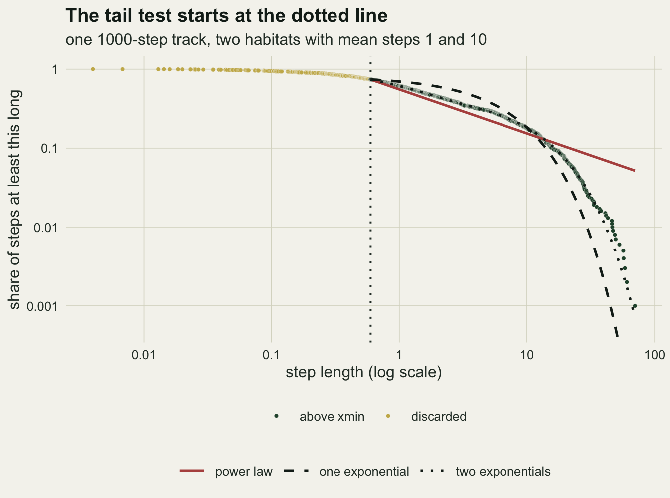
The tail above xmin still holds steps from both habitats. It is a mixture of two exponentials, which on a log-log survival plot is a bent curve; one exponential is a single curve that drops off a cliff, and when the speeds are far enough apart a straight line through the bend fits better than the cliff. So protocol 1 turns on whether the xmin scan leaves more than one speed in the tail, and on how far apart those speeds are.
Call rates by cell
n_track <- 200
se_max  <- sqrt(0.25 / n_track)
set.seed(6021)
sim_list <- list()
for (n_step in c(1000, 300)) {
  for (i in seq_len(nrow(cell_tab))) {
    res <- t(replicate(n_track, score_track(draw_cell(i, n_step))))
    sim_list[[length(sim_list) + 1]] <- data.frame(res, cell = cell_tab$cell[i],
                                                   n_step = n_step)
  }
}
sim_all <- do.call(rbind, sim_list)
sim_all$call_seq <- sim_all$call_mix * (1 - sim_all$lag1)

rate_tab <- aggregate(cbind(call_exp, call_mix, whole_pl, lag1, call_seq) ~ cell + n_step,
                      data = sim_all, FUN = mean)
med_tab  <- aggregate(cbind(n_tail, mu, xmin) ~ cell + n_step, data = sim_all, FUN = median)
rate_tab <- merge(rate_tab, med_tab, by = c("cell", "n_step"))

get_rate <- function(cell_name, n_step, col) {
  rate_tab[rate_tab$cell == cell_name & rate_tab$n_step == n_step, col]
}
mc_se <- function(p) sqrt(p * (1 - p) / n_track)

brown <- cell_tab$cell[1:8]
disc  <- cell_tab$cell[1:3]
cont  <- cell_tab$cell[4:6]
max_whole_brown <- max(rate_tab$whole_pl[rate_tab$cell %in% brown])
levy_whole      <- range(rate_tab$whole_pl[rate_tab$cell == "Levy, mu 2"])
disc_exp_1000 <- sapply(disc, get_rate, n_step = 1000, col = "call_exp")
disc_exp_300  <- sapply(disc, get_rate, n_step = 300,  col = "call_exp")
disc_mix_1000 <- sapply(disc, get_rate, n_step = 1000, col = "call_mix")
disc_mix_300  <- sapply(disc, get_rate, n_step = 300,  col = "call_mix")
cont_exp_1000 <- sapply(cont, get_rate, n_step = 1000, col = "call_exp")
cont_exp_300  <- sapply(cont, get_rate, n_step = 300,  col = "call_exp")
cont_mix_1000 <- sapply(cont, get_rate, n_step = 1000, col = "call_mix")
cont_mix_300  <- sapply(cont, get_rate, n_step = 300,  col = "call_mix")
ntail_1000 <- range(rate_tab$n_tail[rate_tab$n_step == 1000 & rate_tab$cell %in% brown])
ntail_300  <- range(rate_tab$n_tail[rate_tab$n_step == 300 & rate_tab$cell %in% brown])
mix_iidg   <- sapply(c(1000, 300), function(n) get_rate("iid gamma 1.5", n, "call_mix"))
exp_iidg   <- sapply(c(1000, 300), function(n) get_rate("iid gamma 1.5", n, "call_exp"))
Each cell was run 200 times at each track length, a replication fixed before the simulation ran. The denominator throughout is tracks: a rate is the share of the 200 simulated tracks in which a protocol calls Levy, picks the power law, or rejects at lag one, never a share of steps. The Monte Carlo standard error of any rate is at most 0.035.
At 1000 steps protocol 1 calls the discrete-habitat walkers Levy in 0.050 (1 against 5), 0.155 (1 against 10) and 0.160 (three habitats) of tracks. For the continuous cells the rates are 0.765 for the lognormal, 0.545 for the gamma rate with shape 3 and 0.900 for shape 1.5. So the false call is rare with a few discrete habitats and common with continuous speed heterogeneity. Continuity is not the whole story, though. In this set of cells the ordering follows the spread of the patch mean steps: their coefficient of variation is 0.67, 0.82 and 0.78 in the discrete cells, 1.00 for the gamma rate with shape 3, 1.31 for the lognormal and infinite for shape 1.5, and the call rate climbs with it apart from a near tie between the second and third discrete cells.
Adding the mixture as an alternative removes nearly all of the discrete-habitat calls: protocol 2 leaves 0.000, 0.000 and 0.005. It does much less for continuous speeds, which keep 0.185, 0.155 and 0.345. A finite track with around fifty patches has a realised marginal that is a finite mixture, and a two-exponential fit catches it in most tracks even when the generating distribution of speeds is continuous; it does not catch it in all of them. Redrawing the same gamma speeds at every step, so that the track samples the continuous distribution rather than about fifty patches, raises protocol 2 from 0.345 to 0.885.
The whole-range comparison, protocol 3, never picks the power law for any Brownian cell: the largest rate over all eight cells and both lengths is 0.000, against 0.995 to 1.000 for the true Levy walker. That zero is structural rather than clever. A pure power law from the smallest step puts most of its mass just above that step, and exponential steps have a flat head that a power law from the minimum cannot fit. The same flat head is why protocol 3 also rejects the iid gamma cell, whose marginal is a Lomax law with a genuine power-law tail.
h2_sub   <- sim_all[sim_all$cell == "2 habitats, 1:10" & sim_all$n_step == 1000, ]
h2_sub$discard <- 1 - h2_sub$n_tail / 1000
n_h2_call <- sum(h2_sub$call_exp)
qd_call  <- median(h2_sub$discard[h2_sub$call_exp == 1])
qd_unc   <- median(h2_sub$discard[h2_sub$call_exp == 0])
mu_call  <- median(h2_sub$mu[h2_sub$call_exp == 1])
mu_unc   <- median(h2_sub$mu[h2_sub$call_exp == 0])
cap_300  <- 1 - min_tail / 300
brown_rows <- rate_tab[rate_tab$cell %in% brown, ]
over_fac <- range(brown_rows$n_step / brown_rows$n_tail)
Why the discrete cells fool protocol 1 only sometimes is visible in the tracks it calls. In the two-habitat cell with means 1 and 10 at 1000 steps, the 31 called tracks had a median of 38 per cent of steps discarded below xmin and a median exponent of 1.68; the uncalled tracks discarded 86 per cent with a median exponent of 3.06. When the scan cuts high, only the long steps of the fast habitat survive, the tail is one exponential and the exponential wins. When it cuts low, both speeds are in the tail and the power law wins. For discrete habitats it is not the discarded head that hides the mixture: the call happens when the scan keeps the part of the data where the mixture shows.
Shorter tracks push the discrete cells up. At 300 steps protocol 1 calls them Levy in 0.270, 0.395 and 0.300 of tracks, more than at 1000 steps, while protocol 2 leaves 0.060, 0.010 and 0.070. Part of the reason is the design floor of 50 tail steps: at 300 steps xmin cannot sit above the 0.83 quantile, so the high cut that saves the 1000-step tracks is out of reach. The continuous cells move the other way under protocol 1, to 0.580, 0.390 and 0.615; under protocol 2 the lognormal and shape 3 cells barely move, to 0.205 and 0.155, while shape 1.5 falls to 0.240. The tails are also small: the median number of steps above xmin across the Brownian cells is 160 to 240 at 1000 steps and 95 to 141 at 300, and that, not the track length, is the sample size behind every tail rate.
rate_long <- rbind(
  data.frame(rate_tab[, c("cell", "n_step")], rate = rate_tab$call_exp,
             protocol = "tail: power law vs one exponential"),
  data.frame(rate_tab[, c("cell", "n_step")], rate = rate_tab$call_mix,
             protocol = "tail: also vs two exponentials"),
  data.frame(rate_tab[, c("cell", "n_step")], rate = rate_tab$whole_pl,
             protocol = "whole range: power law best of three"),
  data.frame(rate_tab[, c("cell", "n_step")], rate = rate_tab$call_seq,
             protocol = "tail vs two exponentials, then lag-1"))
rate_long$protocol <- factor(rate_long$protocol, levels = unique(rate_long$protocol))
rate_long$cell     <- factor(rate_long$cell, levels = cell_tab$cell)
rate_long$n_lab    <- factor(paste(rate_long$n_step, "steps per track"),
                             levels = c("1000 steps per track", "300 steps per track"))
rate_long$se <- mc_se(rate_long$rate)
ggplot(rate_long, aes(cell, rate, colour = protocol, shape = protocol)) +
  geom_errorbar(aes(ymin = pmax(rate - 2 * se, 0), ymax = pmin(rate + 2 * se, 1)),
                width = 0, linewidth = 0.5, position = position_dodge(width = 0.6)) +
  geom_point(size = 2, position = position_dodge(width = 0.6)) +
  geom_vline(xintercept = c(3.5, 6.5), colour = te_line, linewidth = 0.8) +
  facet_wrap(~n_lab, ncol = 1) +
  scale_colour_manual(values = c(te_rust, te_gold, te_body, te_forest), name = NULL) +
  scale_shape_manual(values = c(16, 15, 1, 17), name = NULL) +
  scale_y_continuous(limits = c(0, 1)) +
  guides(colour = guide_legend(ncol = 2), shape = guide_legend(ncol = 2)) +
  labs(x = NULL, y = "share of tracks called Levy",
       title = "Which test calls a Brownian walker a Levy walker",
       subtitle = "left: discrete habitats; middle: continuous speeds; right: controls") +
  theme_datasheet() +
  theme(legend.position = "bottom",
        axis.text.x = element_text(angle = 35, hjust = 1))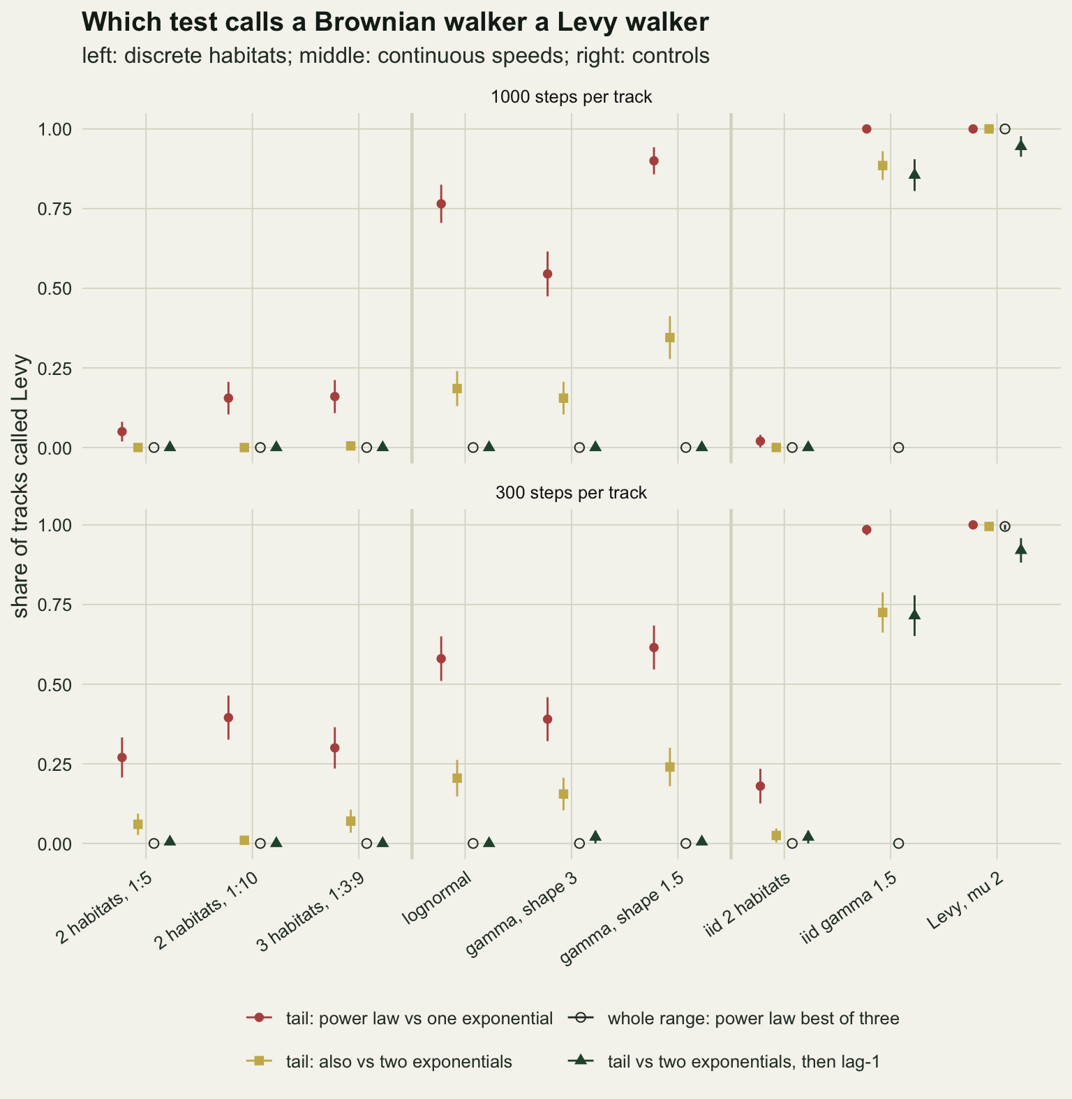
The gamma cells build the power law in
The gamma cells are where a Levy verdict is hardest to argue with on the marginal, because their expected marginal is a power law in the tail. The Lomax closed form predicts the tail exponent, a + 1, and the fitted exponent can be set against it. The prediction is a limit, though: the log-log slope of the Lomax density at a step length x is minus (a + 1) x / (x + a), which only reaches its limit far out in the tail. A fit that starts at a finite xmin sees a shallower slope, and its expected value can be computed for each track’s own xmin by integrating the Lomax survival function above it.
lomax_limit <- function(xm, a) {
  inner <- integrate(function(x) ((1 + x / a) / (1 + xm / a))^(-a) / x,
                     lower = xm, upper = Inf)$value
  1 + 1 / inner
}
exp_cells <- c("gamma, shape 3", "gamma, shape 1.5", "iid gamma 1.5", "Levy, mu 2")
exp_shape <- c(3, 1.5, 1.5, NA)
mu_df <- sim_all[sim_all$cell %in% exp_cells, c("cell", "n_step", "mu", "xmin")]
mu_df$shape  <- exp_shape[match(mu_df$cell, exp_cells)]
mu_df$limit  <- ifelse(is.na(mu_df$shape), 2, mu_df$shape + 1)
mu_df$finite <- ifelse(is.na(mu_df$shape), 2,
                       mapply(function(xm, a) if (is.na(a)) 2 else lomax_limit(xm, a),
                              mu_df$xmin, mu_df$shape))
mu_sum <- aggregate(cbind(mu, finite, limit, xmin) ~ cell + n_step, data = mu_df,
                    FUN = median)
get_mu <- function(cell_name, n_step, col) {
  mu_sum[mu_sum$cell == cell_name & mu_sum$n_step == n_step, col]
}
slope_at <- function(x, a) (a + 1) * x / (x + a)
ga_1000  <- mu_sum[mu_sum$n_step == 1000 & mu_sum$cell != "Levy, mu 2", ]
gap_fin  <- range(ga_1000$mu - ga_1000$finite)
gap_lim  <- range(ga_1000$limit - ga_1000$mu)
ga3_in_1000 <- mean(mu_df$mu[mu_df$cell == "gamma, shape 3" & mu_df$n_step == 1000] > 1 &
                   mu_df$mu[mu_df$cell == "gamma, shape 3" & mu_df$n_step == 1000] <= 3)
At 1000 steps the median fitted exponent is 2.23 in the persistent gamma cell with shape 1.5, against a limit of 2.5 and a finite-xmin expectation of 2.13. For shape 3 the fit is 2.76 against a limit of 4.0 and an expectation of 2.62, and for the iid gamma cell 2.18 against 2.5 and 2.16. At the median xmin of the shape 3 cell, 2.12, the local slope is only 1.65. The true Levy walker returns 2.00, as it should.
So an exponent near 2 in these cells is not a sign that the walker is close to the optimal Levy searcher. It is the Lomax limit dragged down by a finite xmin. The shape 3 cell makes the point most plainly: its limit of 4 is outside the Levy range, and its median fitted exponent sits inside it, as do the exponents of 0.755 of its 1000-step tracks. Reading the fitted exponent as the property of a search rule, rather than of where the scan happened to cut, is the second trap the tail test sets.
mu_df$cell    <- factor(mu_df$cell, levels = exp_cells)
mu_sum$cell   <- factor(mu_sum$cell, levels = exp_cells)
mu_df$n_lab   <- factor(paste(mu_df$n_step, "steps"), levels = c("1000 steps", "300 steps"))
mu_sum$n_lab  <- factor(paste(mu_sum$n_step, "steps"), levels = c("1000 steps", "300 steps"))
mu_sum$x_pos  <- as.numeric(mu_sum$cell)
ggplot(mu_df, aes(cell, mu)) +
  geom_jitter(width = 0.15, height = 0, size = 0.7, alpha = 0.35, colour = te_forest) +
  geom_segment(data = mu_sum, aes(x = x_pos - 0.35, xend = x_pos + 0.35,
                                  y = limit, yend = limit),
               colour = te_rust, linewidth = 1) +
  geom_segment(data = mu_sum, aes(x = x_pos - 0.35, xend = x_pos + 0.35,
                                  y = finite, yend = finite),
               colour = te_gold, linewidth = 1, linetype = "dashed") +
  geom_point(data = mu_sum, aes(y = mu), shape = 23, size = 3, fill = te_ink,
             colour = te_paper) +
  facet_wrap(~n_lab) +
  coord_cartesian(ylim = c(1, 5)) +
  labs(x = NULL, y = "fitted tail exponent mu",
       title = "The fitted exponent sits below the Lomax limit",
       subtitle = paste0("red: limit a + 1; gold dashed: expected fit above each ",
                         "track's own xmin; diamonds: medians")) +
  theme_datasheet() +
  theme(axis.text.x = element_text(angle = 25, hjust = 1))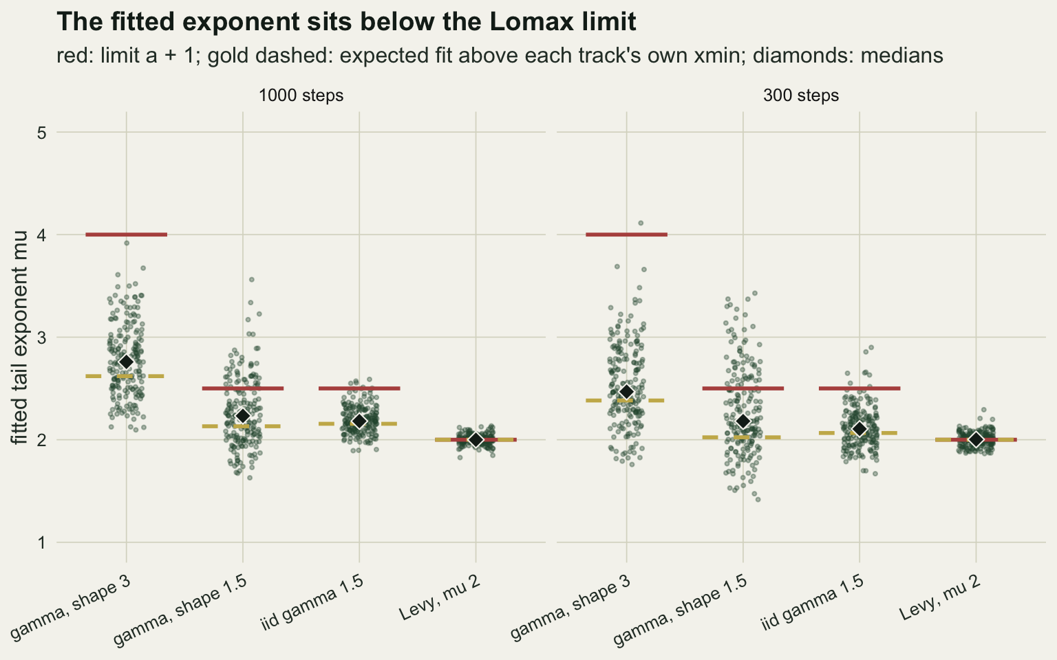
The order of the steps
A persistent walker and an iid walker with the same distribution of speeds have the same expected marginal. What the persistent one has in addition is order: a long step tends to follow a long step, because both were taken in the same patch. The HMM checking post uses exactly this to condemn its one-state model, and the connection to the test here is exact. Its one-state pseudo-residual is qnorm(pgamma(step)), a monotone increasing function of the step, so the ranks of the residuals are the ranks of the steps, and a Spearman lag-one correlation of the raw steps equals the Spearman lag-one correlation of those residuals. The HMM post reports the Pearson lag-one autocorrelation of the residuals, the non-rank version of the same check.
pearson_pred <- function(m_vals) {
  v_m <- mean(m_vals^2) - mean(m_vals)^2
  (1 - q_switch) * v_m / (mean(m_vals^2) + v_m)
}
pred_tab <- data.frame(cell = disc, pred = c(pearson_pred(c(1, 5)),
                                             pearson_pred(c(1, 10)),
                                             pearson_pred(c(1, 3, 9))))
pred_tab$sim <- sapply(disc, function(cn)
  mean(sim_all$pearson1[sim_all$cell == cn & sim_all$n_step == 1000]))
pred_tab$sim_se <- sapply(disc, function(cn)
  sd(sim_all$pearson1[sim_all$cell == cn & sim_all$n_step == 1000]) / sqrt(n_track))
pred_z <- max(abs(pred_tab$sim - pred_tab$pred) / pred_tab$sim_se)
pers <- cell_tab$cell[1:6]
lag_pers_1000 <- range(rate_tab$lag1[rate_tab$n_step == 1000 & rate_tab$cell %in% pers])
lag_pers_300  <- range(rate_tab$lag1[rate_tab$n_step == 300 & rate_tab$cell %in% pers])
lag_ga3_300   <- get_rate("gamma, shape 3", 300, "lag1")
iid_cells     <- cell_tab$cell[7:9]
lag_iid       <- range(rate_tab$lag1[rate_tab$cell %in% iid_cells])

n_null <- 20000
set.seed(4417)
null_p <- sapply(c(1000, 300), function(n_step) {
  mean(replicate(n_null, lag1_test((1 - runif(n_step))^(-1))[["p"]] < 0.05))
})
null_se <- sqrt(null_p * (1 - null_p) / n_null)

seq_pers <- max(rate_tab$call_seq[rate_tab$cell %in% pers])
seq_iidg <- sapply(c(1000, 300), function(n) get_rate("iid gamma 1.5", n, "call_seq"))
seq_levy <- sapply(c(1000, 300), function(n) get_rate("Levy, mu 2", n, "call_seq"))
For the discrete cells the Pearson lag-one correlation of the steps has a closed form. Within a patch the mean step is m and the variance m squared; the patch carries over to the next step with probability 1 - q, so the covariance of successive steps is (1 - q) times the variance of m, and the correlation is (1 - q) var(m) / (E(m squared) + var(m)). That gives 0.224, 0.272 and 0.262 for the three discrete cells, and the simulated means at 1000 steps are 0.222, 0.265 and 0.258, within 1.7 standard errors, slightly low as a lag-one estimate is in a finite series. A correlation of that size on 1000 steps is many standard errors from zero, so the near-certain rejection below is predictable before any test is run.
The lowest rejection rate of the Spearman test in any persistent cell is 1.000 at 1000 steps; at 300 steps the persistent cells run from 0.760 to 0.990, the low end being the gamma cell with shape 3 at 0.760, whose rank correlations sit closest to zero in the figure below. In the three iid cells it rejects in 0.025 to 0.075.
The calibration question has a clean answer. The ranks of any iid sequence from a continuous distribution are a uniformly random permutation, so the null distribution of the rank statistic is the same for exponential, Lomax or Pareto steps; heavy tails cannot miscalibrate it. What remains is whether the t approximation holds for a serial correlation, whose pairs overlap. On 20000 iid Pareto tracks the rejection rate at the nominal 5 per cent is 0.0467 at 1000 steps and 0.0445 at 300, with Monte Carlo standard errors of 0.0015 and 0.0015: slightly conservative, and not by enough to matter.
r_crit <- function(n_step) {
  t_c <- qt(0.95, n_step - 3)
  t_c / sqrt(n_step - 3 + t_c^2)
}
lag_df <- sim_all[, c("cell", "n_step", "rho")]
lag_df$cell  <- factor(lag_df$cell, levels = rev(cell_tab$cell))
lag_df$kind  <- ifelse(lag_df$cell %in% cell_tab$cell[1:6], "persistent patches",
                       "no persistence")
lag_df$n_lab <- factor(paste(lag_df$n_step, "steps"), levels = c("1000 steps", "300 steps"))
crit_df <- data.frame(n_lab = factor(c("1000 steps", "300 steps"),
                                     levels = levels(lag_df$n_lab)),
                      r_c = c(r_crit(1000), r_crit(300)))
ggplot(lag_df, aes(rho, cell, colour = kind)) +
  geom_jitter(width = 0, height = 0.25, size = 0.6, alpha = 0.45) +
  geom_vline(data = crit_df, aes(xintercept = r_c), colour = te_ink,
             linetype = "dashed", linewidth = 0.6) +
  geom_vline(xintercept = 0, colour = te_body, linewidth = 0.3) +
  facet_wrap(~n_lab) +
  scale_x_continuous(breaks = c(0, 0.25, 0.5, 0.75)) +
  scale_colour_manual(values = c("persistent patches" = te_forest,
                                 "no persistence" = te_rust), name = NULL) +
  guides(colour = guide_legend(override.aes = list(size = 2.5, alpha = 1))) +
  labs(x = "lag-1 Spearman correlation of successive steps", y = NULL,
       title = "Order is what the marginal cannot hold",
       subtitle = "one point per track; dashed: one-sided 5 per cent critical value") +
  theme_datasheet() +
  theme(legend.position = "bottom", panel.spacing = unit(1.5, "lines"))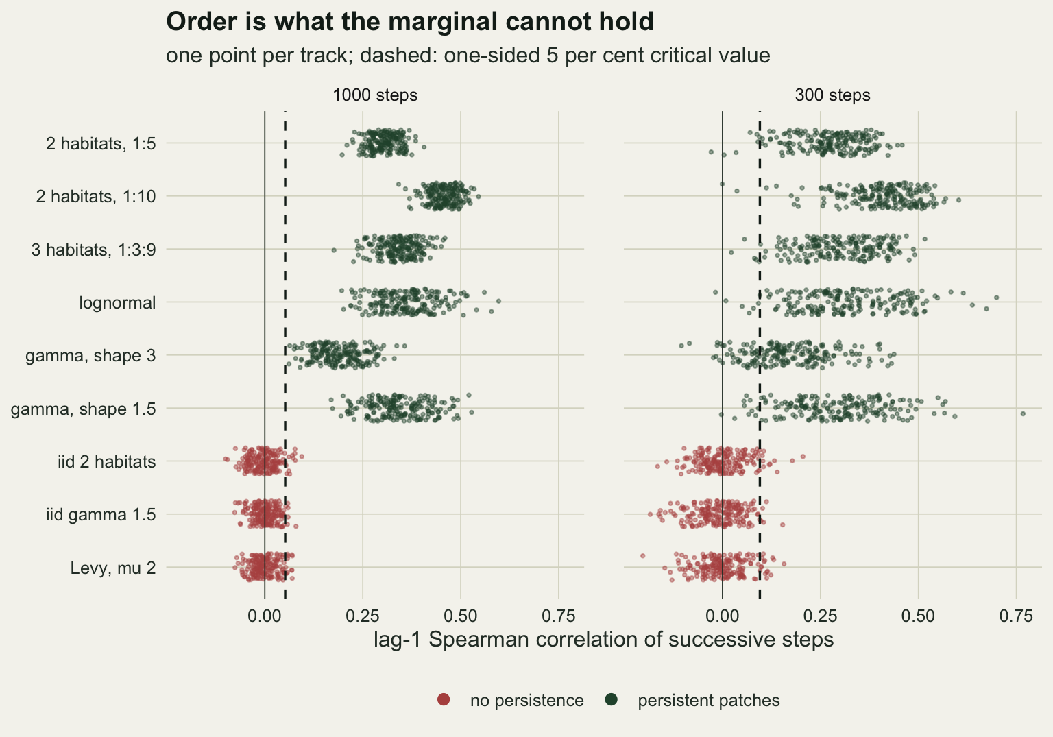
Run in sequence, protocol 2 followed by the serial check, calling Levy only when the power law beats both alternatives on the tail and the lag-one test does not reject, the persistent cells are called Levy in at most 0.020 of tracks at either length. The true Levy walker keeps 0.945 at 1000 steps and 0.920 at 300. The iid gamma walker keeps 0.855 and 0.715, which is almost all of its protocol 2 rate (0.885 and 0.725): a walker whose speed is redrawn at every step, from a gamma distribution heavy enough, passes for a power-law walker on both tail tests (protocol 1 calls it Levy in 1.000 and 0.985), and the serial test finds nothing to separate it; only the whole-range fit rejects it, and that fit would reject a Levy walker with a soft head for the same reason (see Honest limits).
What to report
Report which alternative the power law was compared with, on which range, and where xmin fell. A Levy verdict from a tail against a single exponential says little: with continuous speed heterogeneity that protocol called Brownian walkers Levy in 0.545 to 0.900 of 1000-step tracks here. Put a two-exponential mixture beside the exponential on the same tail, give the share of steps above xmin, and print the AIC differences, not only the winner.
Give the number of steps above xmin as the sample size of the tail fit. The whole track length overstated it by a factor of 2.1 to 6.2 in the Brownian cells here, going by the median tail size per cell.
Report the fitted exponent with the xmin it came from, and do not read it against the optimal value of 2 without asking what a finite xmin does to it. For a Lomax marginal the finite-xmin expectation is one integral. In the gamma cells at 1000 steps the fitted medians sat 0.03 to 0.14 above that expectation and 0.27 to 1.24 below the limit a + 1.
Run the lag-one Spearman test on the raw step series, and say which way it came out. It is distribution free under independence, calibrated on heavy-tailed steps, and at 1000 steps its lowest rejection rate in any persistent cell was 1.000. The order of checks that worked here is: the tail against a mixture as well as an exponential, then the serial test on whatever survives, with the whole-range fit as a description of the head rather than a verdict.
Honest limits
The iid gamma cell is genuine equifinality. A walker that redraws its speed from a heavy gamma distribution at every step has an exactly Lomax marginal and no serial structure, so the power law beats the mixture on the tail in most tracks and the lag-one test cannot see anything. No test on step lengths alone separates it from a Levy walker with a soft head, and only a covariate that tracks the habitat, or the individual, can. The same holds for Petrovskii’s pooled individuals: the pooling is iid by construction.
The composite alternative has two components. For three discrete habitats it was enough in these runs, but whether more components, or an xmin chosen jointly for the power law and the mixture rather than by the power law’s own scan, would shrink the continuous-cell rates further was not measured. A three-component fit also pays eight more AIC units than the power law, for four extra parameters, on a tail of one or two hundred steps.
The true Levy cell is the best case for the whole-range protocol, because Pareto steps are a power law all the way down to their minimum. A real Levy searcher’s short steps are shaped by the fix interval, location error and the resolution of the tag, and rarely follow the power law to the smallest step, so protocol 3 would reject real Levy walkers too; the iid gamma cell shows it doing exactly that to a Lomax law.
Patches here have one length scale, a switching probability of 0.05 per step, and the serial test’s power depends on it. A higher switching probability shrinks the lag-one correlation by the factor 1 - q in the formula above, and a walker that alternates between habitats faster than the fix interval looks iid. The step lengths are also exponential within a patch, the Brownian end of the spectrum; a correlated random walk with gamma steps would change the head and the xmin scan, but not the logic of the mixture comparison.
The xmin scan uses a grid of quantiles and a floor of 50 tail steps. Both are common choices and both move the rates, the floor visibly at 300 steps. Clauset and colleagues also recommend a bootstrap goodness-of-fit test of the power law before any comparison; it was not run here, and how many of the called tracks it would reject is not known from these runs.
References
Benhamou S 2007 Ecology 88(8):1962-1969 (10.1890/06-1769.1)
Petrovskii S, Mashanova A, Jansen VAA 2011 Proceedings of the National Academy of Sciences 108(21):8704-8707 (10.1073/pnas.1015208108)
Jansen VAA, Mashanova A, Petrovskii S 2012 Science 335(6071):918 (comment on de Jager et al. 2011; 10.1126/science.1215747)
Edwards AM, Phillips RA, Watkins NW, Freeman MP, Murphy EJ, Afanasyev V, Buldyrev SV, da Luz MGE, Raposo EP, Stanley HE, Viswanathan GM 2007 Nature 449(7165):1044-1048 (10.1038/nature06199)
Clauset A, Shalizi CR, Newman MEJ 2009 SIAM Review 51(4):661-703 (10.1137/070710111)