Life tables and population growth in R

Build a cohort life table in R and turn age-specific survival and fecundity into R0, generation time and the growth rate lambda via the Euler-Lotka equation.

A life table is the demographic backbone of population ecology. It records, for each age, the chance of surviving and the expected number of offspring, and from those two columns you can read off whether a population grows or shrinks and how fast. This post builds a cohort life table from scratch in R and derives the four numbers that summarise it: the net reproductive rate R0, the generation time T, the intrinsic rate of increase r, and the finite growth rate lambda. The next post rebuilds the same demography as a Leslie matrix and recovers the identical lambda as a matrix eigenvalue.

The two columns that matter

Everything starts from two age-specific schedules. The survival probability from age x to age x+1 we call px; the mean number of female offspring produced by a female of age x we call mx (counting daughters keeps the bookkeeping to one sex). From the survivals we build the survivorship lx, the probability of surviving from birth to the start of age x, as a running product.

library(ggplot2)
library(dplyr)

te_ink <- "#16241d"; te_forest <- "#275139"; te_mown <- "#2f8f63"
te_aband <- "#b5534e"; te_faint <- "#5d6b61"; te_line <- "#dad9ca"; te_paper <- "#f5f4ee"
theme_te <- function(base_size = 12) {
  theme_minimal(base_size = base_size) +
    theme(text = element_text(colour = "#2c3a31"),
          plot.title = element_text(colour = te_ink, face = "bold", size = base_size * 1.15),
          plot.subtitle = element_text(colour = te_faint, size = base_size * 0.95),
          axis.title = element_text(colour = "#46604a"), axis.text = element_text(colour = te_faint),
          panel.grid.minor = element_blank(),
          panel.grid.major = element_line(colour = te_line, linewidth = 0.3),
          plot.background = element_rect(fill = te_paper, colour = NA),
          panel.background = element_rect(fill = te_paper, colour = NA),
          legend.key = element_rect(fill = te_paper, colour = NA))
}

age <- 0:5
px  <- c(0.50, 0.60, 0.70, 0.70, 0.50, 0.00)   # survival from age x to x+1
mx  <- c(0.00, 0.00, 1.50, 2.00, 1.70, 1.00)   # female offspring per female at age x
lx  <- cumprod(c(1, head(px, -1)))             # survivorship to the start of age x
round(lx, 4)

[1] 1.0000 0.5000 0.3000 0.2100 0.1470 0.0735

The population matures at age two, peaks in reproduction at age three, and no individual lives past age five. The survivorship falls steeply early on: only half survive their first year, and about seven percent reach age five.

Reading a life table

Two derived columns do the work. The product lx * mx is the expected reproductive output of a newborn at each age, and x * lx * mx weights that output by age. Summing them gives the two headline quantities.

lxmx <- lx * mx
R0   <- sum(lxmx)                 # net reproductive rate
Tgen <- sum(age * lxmx) / R0      # cohort generation time (mean age of mothers)
data.frame(x = age, px = px, lx = round(lx, 4), mx = mx,
           lxmx = round(lxmx, 4), xlxmx = round(age * lxmx, 4))

  x  px     lx  mx   lxmx  xlxmx
1 0 0.5 1.0000 0.0 0.0000 0.0000
2 1 0.6 0.5000 0.0 0.0000 0.0000
3 2 0.7 0.3000 1.5 0.4500 0.9000
4 3 0.7 0.2100 2.0 0.4200 1.2600
5 4 0.5 0.1470 1.7 0.2499 0.9996
6 5 0.0 0.0735 1.0 0.0735 0.3675

The net reproductive rate R0 is the mean number of daughters a female produces over her whole life. Here it is about 1.19, so each generation replaces itself and adds roughly a fifth. R0 > 1 means growth, R0 < 1 means decline, and R0 = 1 is exact replacement. The generation time T is the mean age of the mothers of a cohort of offspring, close to three years, sitting between the ages that contribute the most reproduction.

From R0 to a growth rate

R0 tells you the per-generation multiplier, but ecologists usually want a per-year rate. The quick conversion divides log R0 by the generation time.

r_approx <- log(R0) / Tgen
c(r_approx = r_approx, lambda_approx = exp(r_approx))

     r_approx lambda_approx 
   0.05982272    1.06164832 

That shortcut gives an intrinsic rate near 0.060 and a finite rate lambda of about 1.062, so the population grows by roughly six percent a year. The shortcut is only approximate because it treats the generation time as if all reproduction happened at a single age. The exact rate comes from the Euler-Lotka equation, which asks for the value of r that makes the discounted lifetime reproduction sum to exactly one.

euler <- function(r) sum(lxmx * exp(-r * age)) - 1
r_exact <- uniroot(euler, interval = c(-1, 1), tol = 1e-12)$root
c(r_exact = r_exact, lambda = exp(r_exact), residual = euler(r_exact))

   r_exact     lambda   residual 
0.06032882 1.06218576 0.00000000 

Solving numerically with uniroot gives r of about 0.0603 and lambda of about 1.062. The residual is effectively zero, confirming the root. The shortcut was off by only about 0.0005 here, but the gap widens when the reproductive schedule is spread across many ages, so the Euler-Lotka value is the one to report.

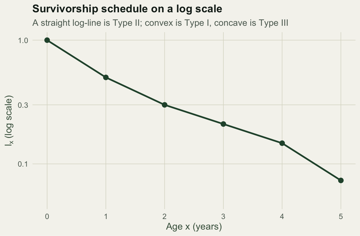
Survivorship on a log scale

Plotting lx on a log axis is the standard diagnostic for survivorship type. A straight line means constant mortality (Type II); a convex curve means most deaths come late (Type I, typical of large mammals); a concave curve means most deaths come early (Type III, typical of species with many offspring and little parental care).

ggplot(data.frame(age = age, lx = lx), aes(age, lx)) +
  geom_line(colour = te_forest, linewidth = 1) +
  geom_point(colour = te_forest, size = 2.6) +
  scale_y_log10(limits = c(0.05, 1)) +
  labs(title = "Survivorship schedule on a log scale",
       subtitle = "A straight log-line is Type II; convex is Type I, concave is Type III",
       x = "Age x (years)", y = expression(l[x] ~ "(log scale)")) +
  theme_te()

Figure 1: Survivorship on a log scale; the shape flags the mortality pattern.

This schedule is concave early and then straightens, a common intermediate pattern: heavy first-year mortality followed by steadier adult survival.

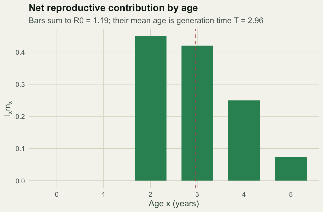
Where the growth comes from

The lx * mx column shows which ages actually drive population growth. Plotting it makes the contribution explicit, and the bars sum to R0.

ggplot(data.frame(age = age, lxmx = lxmx), aes(factor(age), lxmx)) +
  geom_col(fill = te_mown, width = 0.68) +
  geom_vline(xintercept = Tgen + 1, linetype = "dashed", colour = te_aband) +
  labs(title = "Net reproductive contribution by age",
       subtitle = sprintf("Bars sum to R0 = %.2f; their mean age is generation time T = %.2f", R0, Tgen),
       x = "Age x (years)", y = expression(l[x] * m[x])) +
  theme_te()

Figure 2: Net reproductive contribution by age; bars sum to R0 and their mean age is T.

The middle ages carry the population. Early survival matters because it delivers individuals to those reproductive ages, which is exactly the kind of dependence a sensitivity analysis quantifies later in this series.

What to take away

A life table reduces to two schedules, survival and fecundity, and four summary numbers. R0 is the per-generation multiplier, T is the average age of reproduction, and r and lambda are the per-year growth rates, with the Euler-Lotka equation giving the exact value. The same information can be arranged as a projection matrix, and the next post shows that the dominant eigenvalue of that matrix equals the lambda derived here.

References

• Lotka AJ 1907 Science 26(653):21-22 (10.1126/science.26.653.21.b)
• Sharpe FR, Lotka AJ 1911 Philosophical Magazine Series 6, 21:435-438 (pre-DOI)
• Cole LC 1954 Quarterly Review of Biology 29(2):103-137 (10.1086/400074)
• Stearns SC 1992 The Evolution of Life Histories, Oxford University Press (ISBN 978-0-19-857741-6)
• Gotelli NJ 2008 A Primer of Ecology, 4th ed, Sinauer (ISBN 978-0-87893-318-1)

Related tutorials

• Leslie matrix population models in R
• Stage-structured Lefkovitch matrices in R
• Sensitivity and elasticity of matrix models
• Bootstrap confidence intervals in R