Independent contrasts: Felsenstein’s method

Phylogenetic independent contrasts in R with ape: turn correlated species data into independent points, regress through the origin, and check branch lengths.

Suppose you have body size and metabolic rate for fifty species and you want the relationship between them. The obvious move, regress one on the other across species, has a hidden flaw: the species are not independent observations. Two close relatives resemble each other because they share ancestry, not because they provide two separate tests of the relationship. Treat them as independent and you count the same evolutionary event many times over, which shrinks your standard errors and can shift the slope.

Felsenstein’s phylogenetically independent contrasts, introduced in 1985, are the classic fix. The idea is to work not with the species values but with the differences between them along the tree. Under Brownian motion, the difference between two sister lineages depends only on the evolution that happened after they split, so these differences are statistically independent of one another. They are the independent data points the raw species values only pretended to be.

Setup

library(ape)
library(nlme)
library(ggplot2)

te_paper <- "#f5f4ee"; te_ink   <- "#16241d"; te_body <- "#2c3a31"
te_faint <- "#5d6b61"; te_sage  <- "#93a87f"; te_rust <- "#b5534e"
te_line  <- "#dad9ca"; te_green <- "#2f8f63"; te_gold <- "#cda23f"

theme_te <- function(base_size = 12) {
  theme_minimal(base_size = base_size) +
    theme(
      plot.background  = element_rect(fill = te_paper, colour = NA),
      panel.background = element_rect(fill = te_paper, colour = NA),
      panel.grid.major = element_line(colour = te_line, linewidth = 0.3),
      panel.grid.minor = element_blank(),
      axis.text  = element_text(colour = te_body),
      axis.title = element_text(colour = te_ink),
      plot.title = element_text(colour = te_ink, face = "bold"),
      strip.text = element_text(colour = te_ink, face = "bold")
    )
}

A tree and two traits

We simulate one ultrametric tree of 50 species and evolve two traits on it. The first, x, evolves by pure Brownian motion. The second, y, evolves partly with x (a true evolutionary slope of 0.75) and partly on its own. Because we set the generating slope ourselves, we can check which method recovers it.

set.seed(1)
tree <- rcoal(50)
tree$tip.label <- sprintf("t%02d", 1:50)
x <- rTraitCont(tree, model = "BM", sigma = 1)
y <- 0.75 * x + rTraitCont(tree, model = "BM", sigma = 0.6)

What a contrast is

At every internal node the tree joins two descendant lineages. A contrast is the difference between their trait values, standardised by the expected amount of divergence, which is the square root of the summed branch lengths connecting them. A tree of n tips has n - 1 internal nodes, so fifty species give forty-nine contrasts. The pic() function in ape computes them.

cx <- pic(x, tree)
cy <- pic(y, tree)
length(cx)

[1] 49

Regression through the origin

Now regress the y contrasts on the x contrasts. One detail matters: the direction of subtraction at each node is arbitrary, so a contrast can be written with either sign as long as both traits use the same direction. That symmetry means the cloud of contrasts is centred on the origin, and the fitted line must pass through it. In R you drop the intercept with - 1.

m_pic <- lm(cy ~ cx - 1)
c(slope = coef(m_pic)[[1]], se = summary(m_pic)$coef[1, 2],
  p = summary(m_pic)$coef[1, 4])

       slope           se            p 
7.536352e-01 8.651360e-02 1.894646e-11 

Compare that with the ordinary regression on the raw species values, which ignores the tree entirely.

m_ols <- lm(y ~ x)
c(slope = coef(m_ols)[[2]], se = summary(m_ols)$coef[2, 2],
  p = summary(m_ols)$coef[2, 4])

       slope           se            p 
1.058053e+00 1.045110e-01 1.690194e-13 

The contrast regression gives a slope of 0.75, right on the generating value of 0.75. The ordinary regression gives 1.06, larger and with a standard error that treats fifty correlated species as fifty independent facts. The difference is not a rounding artefact; it is the shared history being counted as evidence.

rng_x <- range(x); rng_cx <- range(cx)
lev <- c("species values (ordinary regression)", "contrasts (through the origin)")
pts <- rbind(
  data.frame(panel = lev[1], xv = x,  yv = y),
  data.frame(panel = lev[2], xv = cx, yv = cy))
ln <- rbind(
  data.frame(panel = lev[1], xv = rng_x,  yv = coef(m_ols)[1] + coef(m_ols)[2] * rng_x),
  data.frame(panel = lev[2], xv = rng_cx, yv = coef(m_pic)[1] * rng_cx))
pts$panel <- factor(pts$panel, levels = lev)
ln$panel  <- factor(ln$panel,  levels = lev)
ggplot(pts, aes(xv, yv)) +
  geom_point(colour = te_green, alpha = 0.7, size = 1.8) +
  geom_line(data = ln, colour = te_rust, linewidth = 0.9) +
  facet_wrap(~panel, scales = "free") +
  labs(x = "trait x  (or its contrast)", y = "trait y  (or its contrast)",
       title = "From species values to independent contrasts") +
  theme_te(12)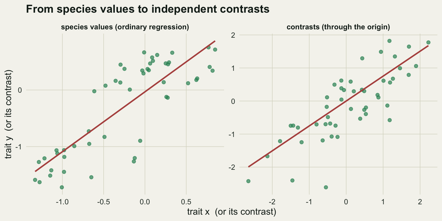

Figure 1: Left: the raw species values with the ordinary regression line, which counts related species as independent. Right: the phylogenetic contrasts with the line forced through the origin, the regression that respects the tree.

Checking the branch lengths

Contrasts are only independent and identically scaled if the branch lengths used to standardise them are adequate. The standard diagnostic plots the absolute value of each standardised contrast against the standard deviation used to standardise it. If the branch lengths do the job, there should be no trend: large and small expected divergences should give contrasts of similar standardised size. A rising or falling trend is a sign that the branch lengths, or the assumed model of evolution, need attention, often a log transform of the trait.

pic_x <- pic(x, tree, var.contrasts = TRUE)
abs_c <- abs(pic_x[, "contrasts"])
sd_c  <- sqrt(pic_x[, "variance"])
ct    <- cor.test(abs_c, sd_c)
c(correlation = unname(ct$estimate), p = ct$p.value)

correlation           p 
 -0.1457109   0.3177997 

ggplot(data.frame(sd_c, abs_c), aes(sd_c, abs_c)) +
  geom_point(colour = te_gold, size = 2, alpha = 0.8) +
  geom_smooth(method = "lm", colour = te_ink, fill = te_sage, alpha = 0.25, linewidth = 0.7) +
  labs(x = "standard deviation of the contrast",
       y = "absolute standardised contrast",
       title = "No trend means the branch lengths are adequate") +
  theme_te(12)

`geom_smooth()` using formula = 'y ~ x'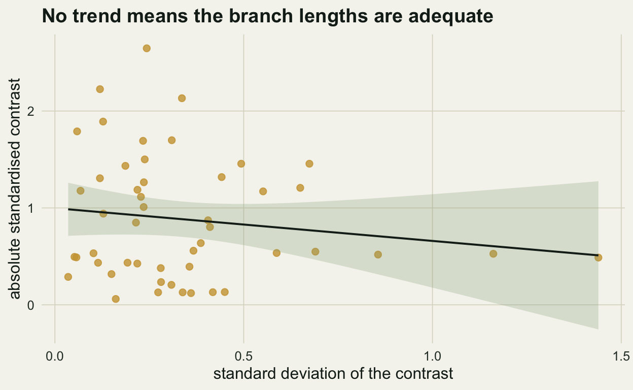

Figure 2: The branch-length check: absolute standardised contrasts against their standard deviation. A flat cloud, as here, means the standardisation is working.

The correlation is -0.15 with a p of 0.32, so there is no evidence the branch lengths are misbehaving.

The payoff: contrasts are least squares in disguise

Here is the result that ties the method to the rest of the comparative toolkit. Regressing contrasts through the origin gives exactly the same slope as phylogenetic generalised least squares with a Brownian correlation structure. They are two computational routes to one estimator.

d <- data.frame(sp = tree$tip.label, x = x[tree$tip.label], y = y[tree$tip.label])
m_pgls <- gls(y ~ x, data = d, correlation = corBrownian(1, tree, form = ~sp))
c(pic_slope  = coef(m_pic)[[1]],
  pgls_slope = coef(m_pgls)[[2]],
  difference = abs(coef(m_pic)[[1]] - coef(m_pgls)[[2]]))

   pic_slope   pgls_slope   difference 
7.536352e-01 7.536352e-01 1.443290e-15 

The two slopes agree to the limits of floating-point arithmetic. Contrasts came first, in 1985, and remain the more transparent way to see why the tree matters; generalised least squares is the more flexible frame, because it lets you estimate how tree-like the residuals really are rather than assuming strict Brownian motion. Knowing they coincide under Brownian motion means you can move between them without changing your answer.

Reading it

A few things are worth keeping straight. Contrasts test the relationship between the traits after removing shared history, so the slope is an evolutionary regression, not a snapshot of living species. The intercept is gone by construction, which is correct for contrasts but means you cannot read a mean trait value off the fit. And the whole apparatus rests on the tree and its branch lengths being roughly right; the diagnostic above is the minimum check, not a guarantee. When the branch-length plot shows a trend, transform the trait or move to a model that estimates the branch scaling, which is the natural cue to reach for phylogenetic signal indices or a fuller least-squares fit.

References

• Felsenstein 1985 The American Naturalist 125(1):1-15 (10.1086/284325)
• Garland, Harvey & Ives 1992 Systematic Biology 41(1):18-32 (10.1093/sysbio/41.1.18)
• Grafen 1989 Philosophical Transactions of the Royal Society B 326(1233):119-157 (10.1098/rstb.1989.0106)
• Paradis & Schliep 2019 Bioinformatics 35(3):526-528 (10.1093/bioinformatics/bty633)

Related tutorials

• Phylogenetic generalised least squares
• Phylogenetic signal: Blomberg’s K and Pagel’s lambda
• Ancestral state reconstruction in R
• Phylogenetic diversity with picante