library(ggplot2)
library(patchwork)

te_paper  <- "#f5f4ee"
te_ink    <- "#16241d"
te_body   <- "#2c3a31"
te_forest <- "#275139"
te_rust   <- "#b5534e"
te_gold   <- "#c9b458"
te_line   <- "#dad9ca"

theme_datasheet <- function() {
  theme_minimal(base_size = 12) +
    theme(plot.background  = element_rect(fill = te_paper, colour = NA),
          panel.background = element_rect(fill = te_paper, colour = NA),
          panel.grid.major = element_line(colour = te_line, linewidth = 0.3),
          panel.grid.minor = element_blank(),
          text             = element_text(colour = te_body),
          plot.title       = element_text(colour = te_ink, face = "bold"),
          plot.subtitle    = element_text(colour = te_body),
          axis.text        = element_text(colour = te_body),
          strip.text       = element_text(colour = te_ink))
}Geolocator latitude near the equinox
R
movement
geolocation
simulation
ecology tutorial
Light-level geolocators turn daylength into latitude. Simulating in R how canopy shading, the equinox and Hill-Ekstrom calibration bend a songbird track.
A wood warbler breeding in a beech forest carries a light logger of well under a gram, fitted with leg loops. It records light intensity every few minutes for a year and is recovered, if the bird returns, the next spring. Everything the logger says about where the bird went comes from two times per day: the moment the light crosses a threshold in the morning and the moment it crosses back in the evening. The midpoint of the two gives solar noon and so longitude. The interval between them gives daylength, and daylength at a known date gives latitude. That second step is the subject here, because it has a known weak point: around the equinoxes daylength is nearly the same at every latitude, and the latitude estimate falls apart. Hill (1994) set out the geometry for tags on elephant seals, and threshold analyses since then have had to decide which days around the equinox to throw away.
The threshold does not correspond to sunrise. It corresponds to a sun elevation angle, usually a few degrees below the horizon, and that angle has to be calibrated: from twilights recorded at a known place, the analyst finds the elevation of the sun at the moments the threshold was crossed. Lisovski et al. (2012) put stationary loggers at known sites and on birds and found that weather adds noise to twilight times, while vegetation and topography shade the sensor and bias the positions; they also found that the choice of calibration method shifts estimated latitudes. Fudickar et al. (2012) measured latitude errors of about 200 km for stationary loggers in forest. The alternative to a calibration site is Hill-Ekstrom calibration (Hill 1994; Ekstrom 2004), which chooses the angle that makes the latitude of a stationary bird flat across the equinox; the user’s guide by Lisovski et al. (2020) describes it and the newer template-fit and state-space methods that are now widely used alongside the plain threshold method. All of this is known, and the post is a demonstration of it with the numbers made explicit.
Daylength as a predictor in ecology builds the daylength formula in base R and uses it forwards, from a known latitude to a covariate; its section “Two practical traps” deals with the twilight coefficient and the polar failure of the arc cosine, but never inverts it for latitude. This post runs the same geometry backwards, the way a geolocator analysis does. A particle filter for animal movement starts from positions that already carry heavy-tailed errors; here the positions are produced, and the error has a sign and a season. And the twilight times themselves are clock readings, which Dates and times in ecological data explains are not instants until a time zone is attached; everything below works in solar hour angles and avoids the question.
The post does four things. It writes the latitude inversion in closed form and checks it against root finding. It shows that the flip of the error across the equinox under a wrong angle is trigonometry, and says where the blind day actually falls. It then adds random, one-sided shading to every twilight and measures what cannot be computed by hand: the share of days with no latitude, and how wide the excluded window around the equinox must be for a given mismatch between calibration and deployment habitat. Last, it applies Hill-Ekstrom calibration, as the published implementations define it, to simulated birds that did not move and to birds that did.
Latitude from daylength in closed form
Declination comes from day of year through the CBM formula compared by Forsythe et al. (1995), the same one used in the daylength post. Elevation angles here follow geolocator practice: negative below the horizon, so an angle of -4 is the sun four degrees down. At latitude phi, declination d and elevation a, the hour angle H of the threshold crossing satisfies sin a = sin phi sin d + cos phi cos d cos H. With H known from the logged daylength, the right side is A sin phi + B cos phi with A = sin d and B = cos d cos H, which is R cos(phi - psi) with R the length of (A, B) and psi its angle. So phi = psi plus or minus acos(sin a / R).
That gives two candidate latitudes, or none when sin a / R lies outside the range of a cosine. The function below keeps only roots in the northern hemisphere, since an analyst tracking a European breeder knows which hemisphere the bird starts in. A day with one northern root has a latitude. A day with no root, or with two northern roots and nothing in the data to choose between them, has none, and the function records which of the two failures happened.
rad <- pi / 180
declination <- function(doy) {
  theta <- 0.2163108 + 2 * atan(0.9671396 * tan(0.00860 * (doy - 186)))
  asin(0.39795 * cos(theta))
}
equinox <- uniroot(declination, c(250, 280), tol = 1e-8)$root

hour_angle <- function(lat, decl, elev) {
  arg <- (sin(elev * rad) - sin(lat * rad) * sin(decl)) /
    (cos(lat * rad) * cos(decl))
  arg[abs(arg) > 1] <- NA
  acos(arg)
}

lat_roots <- function(half_day, decl, elev) {
  a_part <- sin(decl)
  b_part <- cos(decl) * cos(half_day)
  r_len  <- sqrt(a_part^2 + b_part^2)
  psi    <- atan2(a_part, b_part)
  ratio  <- sin(elev * rad) / r_len
  spread <- acos(pmin(1, pmax(-1, ratio)))
  wrap   <- function(x) (x + pi) %% (2 * pi) - pi
  root_1 <- wrap(psi + spread) / rad
  root_2 <- wrap(psi - spread) / rad
  ok_1 <- abs(ratio) <= 1 & root_1 > 0 & root_1 < 90
  ok_2 <- abs(ratio) <= 1 & root_2 > 0 & root_2 < 90
  ok_1[is.na(ok_1)] <- FALSE
  ok_2[is.na(ok_2)] <- FALSE
  lat <- ifelse(ok_1 & !ok_2, root_1, ifelse(ok_2 & !ok_1, root_2, NA))
  status <- ifelse(ok_1 & ok_2, "two roots",
                   ifelse(ok_1 | ok_2, "one root", "no root"))
  status[is.na(half_day)] <- "no root"
  list(lat = lat, status = status)
}
lat_north <- function(half_day, decl, elev) lat_roots(half_day, decl, elev)$lat

set.seed(5210)
n_check <- 2000
chk_lat  <- runif(n_check, 30, 65)
chk_doy  <- sample(c(181:255, 280:351), n_check, replace = TRUE)
chk_elev <- runif(n_check, -7, -1)
chk_dec  <- declination(chk_doy)
chk_half <- hour_angle(chk_lat, chk_dec, chk_elev)
closed   <- lat_north(chk_half, chk_dec, chk_elev)
by_root  <- mapply(function(h, dcl, el) {
  f <- function(p) hour_angle(p, dcl, el) - h
  grid_p <- seq(0.5, 75, by = 0.5)
  vals <- sapply(grid_p, f)
  cross <- which(!is.na(vals[-1]) & !is.na(vals[-length(vals)]) &
                   sign(vals[-1]) != sign(vals[-length(vals)]))
  if (length(cross) != 1) return(NA)
  uniroot(f, grid_p[c(cross, cross + 1)], tol = 1e-10)$root
}, chk_half, chk_dec, chk_elev)
both_ok <- !is.na(closed) & !is.na(by_root)
root_gap <- max(abs(closed[both_ok] - by_root[both_ok]))
n_both <- sum(both_ok)
On 1966 of 2000 random cases (latitudes 30 to 65 N, elevation angles -7 to -1, days away from the autumn equinox) both the closed form and a bracketed root search returned a unique northern latitude, and the largest difference between them was 2.49e-11 degrees. The declination formula puts the autumn equinox at day 266.65, and days below are counted from it.
The flip across the equinox is trigonometry
Shading makes the light threshold arrive later in the morning and earlier in the evening, which is the same as a sun elevation angle higher than the calibrated one. Fix a bird at 52 N with a true angle of -4, let the logger see the world through an angle raised by a constant offset, and invert with the unshaded angle. There is no noise in this chunk.
elev_true <- -4
lat_home  <- 52
km_deg    <- 111.2
days      <- 181:351
day_eq    <- days - equinox
offsets   <- c(0.5, 1, 2)
flip_df <- do.call(rbind, lapply(offsets, function(off) {
  half <- hour_angle(lat_home, declination(days), elev_true + off)
  data.frame(offset = off, doy = days, from_eq = day_eq,
             err_km = km_deg * (lat_north(half, declination(days), elev_true) - lat_home))
}))
far_2 <- flip_df[flip_df$offset == 2 & abs(flip_df$from_eq) > 21, ]
far_2$scaled <- abs(far_2$err_km * tan(declination(far_2$doy)))
scaled_pre  <- range(far_2$scaled[far_2$from_eq < 0])
scaled_post <- range(far_2$scaled[far_2$from_eq > 0])
flip_at <- function(off, t) flip_df$err_km[flip_df$offset == off & round(flip_df$from_eq) == t][1]
blind_day_for <- function(elev, lat = lat_home) {
  target <- asin(sin(elev * rad) * sin(lat * rad))
  uniroot(function(x) declination(x) - target, c(equinox, 320))$root - equinox
}
blind_decl <- asin(sin(elev_true * rad) * sin(lat_home * rad))
blind_day  <- blind_day_for(elev_true)
blind_sunrise <- blind_day_for(-0.833)
blind_six     <- blind_day_for(-6)
n_missing_2 <- sum(is.na(flip_df$err_km[flip_df$offset == 2]))
missing_span <- range(flip_df$from_eq[flip_df$offset == 2 & is.na(flip_df$err_km)])
A shorter day in late summer, when days are still long in the north, reads as a place nearer the equator; a shorter day later in autumn reads as a place nearer the pole. The switch between the two is not quite the equinox but the blind day a little after it, explained below. With an offset of 2 degrees the error is -628 km thirty days before the equinox and +807 km thirty days after it. With an offset of half a degree the same pair is -143 and +228 km. If the error grew exactly as 1/tan(d), the absolute error times the absolute tangent of the declination would be constant. Beyond three weeks at the 2 degree offset it runs from 117 to 139 km before the equinox and from 158 to 175 km after it, so 1/tan(d) describes the growth only roughly, and the two sides differ.
They differ because the blind day is not the equinox. Setting the derivative of daylength with respect to latitude to zero gives sin d = sin a sin phi, so the blind day depends on the sun elevation angle as well as on latitude. For an angle of -4 at 52 N that is a declination of -3.15 degrees, reached 8.1 days after the autumn equinox. Before the equinox the twilight and the geometry both lengthen the day towards the pole; after it they pull in opposite directions and cancel on the blind day. With the 2 degree offset the inversion returned no latitude on 11 days, all between -0.7 and 9.3 days from the equinox. Because the sun elevation angle is below the horizon, this dead zone sits almost entirely after the autumn equinox (and before the spring one), and it moves further from the equinox for a lower angle or a higher latitude: at 52 N the blind day comes 1.7 days after the autumn equinox for the standard sunrise angle of -0.833 and 12.2 days after it for an angle of -6.
ggplot(flip_df, aes(from_eq, err_km, colour = factor(offset))) +
  geom_hline(yintercept = 0, colour = te_body, linewidth = 0.4) +
  geom_vline(xintercept = 0, colour = te_body, linewidth = 0.4) +
  geom_vline(xintercept = blind_day, colour = te_body, linetype = "dotted",
             linewidth = 0.6) +
  geom_line(linewidth = 0.9, na.rm = TRUE) +
  scale_colour_manual(values = c("0.5" = te_gold, "1" = te_forest, "2" = te_rust),
                      name = "angle offset (degrees)") +
  coord_cartesian(ylim = c(-3000, 3000)) +
  labs(x = "days from the autumn equinox", y = "latitude error (km, north positive)",
       title = "South before the equinox, north after it",
       subtitle = "bird at 52 N, true angle -4, no noise") +
  theme_datasheet() +
  theme(legend.position = "bottom")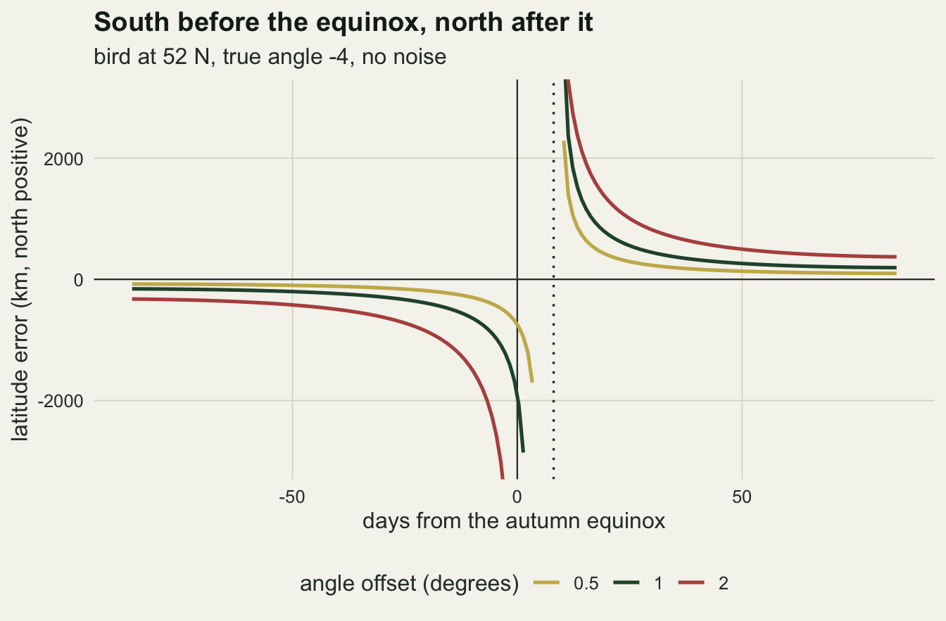
Random shading and the days with no latitude
A constant offset is what a calibration can remove. Real shading is not constant: a bird roosting inside a hedge one night and on an open branch the next shades each twilight by a different amount, and the amount is never negative. Each twilight below gets its own shading, drawn from an exponential distribution in degrees of elevation, independently for sunrise and sunset. The calibration angle is the median sun elevation over 40 twilights recorded at the known site in the 20 days before deployment (days 161 to 180), and the bird then stays at 52 N from day 181 to day 351. These constants were fixed before the first run.
Three scenarios, each with 1000 simulated birds: calibration in the open (mean shading 0.5 degrees, a logger on a post at the capture site) and deployment in forest (mean 2 degrees); calibration and deployment both in forest; and both in the open.
n_bird    <- 1000
cal_days  <- 161:180
simulate_half_days <- function(doys, shade_mean, n, lat = lat_home) {
  n_d  <- length(doys)
  dcl  <- matrix(declination(doys), n, n_d, byrow = TRUE)
  rise <- elev_true + matrix(rexp(n * n_d, 1 / shade_mean), n)
  sets <- elev_true + matrix(rexp(n * n_d, 1 / shade_mean), n)
  latm <- matrix(lat, n, n_d, byrow = TRUE)
  list(half = (hour_angle(latm, dcl, rise) + hour_angle(latm, dcl, sets)) / 2,
       decl = dcl, elev = cbind(rise, sets))
}
calibrate <- function(shade_mean, n) {
  apply(simulate_half_days(cal_days, shade_mean, n)$elev, 1, median)
}
run_scenario <- function(cal_shade, dep_shade, n = n_bird) {
  a_cal <- calibrate(cal_shade, n)
  dep   <- simulate_half_days(days, dep_shade, n)
  fit   <- lat_roots(dep$half, dep$decl, matrix(a_cal, n, length(days)))
  list(err = matrix(km_deg * (fit$lat - lat_home), n),
       status = matrix(fit$status, n), a_cal = a_cal)
}
set.seed(2012)
scen <- list(open_shaded = run_scenario(0.5, 2),
             same_shaded = run_scenario(2, 2),
             open_open   = run_scenario(0.5, 0.5))
pre_far  <- day_eq < -21
post_far <- day_eq > 21
sc_med <- function(s, cols) median(scen[[s]]$err[, cols], na.rm = TRUE)
sc_mad <- function(s, cols) mad(scen[[s]]$err[, cols], na.rm = TRUE)
sc_fail <- function(s, cols, what = c("no root", "two roots")) mean(scen[[s]]$status[, cols] %in% what)
near  <- abs(day_eq) <= 3
post_3_14 <- day_eq > 3 & day_eq <= 14
band_14_21 <- abs(day_eq) > 14 & abs(day_eq) <= 21
a_cal_open <- median(scen$open_shaded$a_cal)
a_cal_same <- median(scen$same_shaded$a_cal)

day_summary <- do.call(rbind, lapply(names(scen), function(s) {
  e <- scen[[s]]$err
  data.frame(scenario = s, from_eq = day_eq,
             med = apply(e, 2, median, na.rm = TRUE),
             lo = apply(e, 2, quantile, 0.25, na.rm = TRUE),
             hi = apply(e, 2, quantile, 0.75, na.rm = TRUE),
             no_root = colMeans(scen[[s]]$status == "no root"),
             two_roots = colMeans(scen[[s]]$status == "two roots"))
}))
The open calibration returns a median angle of -3.65 and the forest calibration -2.60. With the open angle applied to a forest bird, the median error more than three weeks before the equinox is -277 km and more than three weeks after it +349 km. That is the flip of the previous section, now carried by the median of noisy days: the random part of the shading averages into a constant offset, and the calibration in the open did not see it. When the calibration comes from the same habitat, the pair shrinks to -55 and +71 km, but the spread does not: the median absolute deviation of daily errors beyond three weeks is 260 km before the equinox and 326 km after, against 61 and 87 km for a bird in the open. Between 14 and 21 days from the equinox the same-habitat spread is 710 km. Matching the habitat removes most of the bias and leaves the noise, and in forest the noise alone is a few hundred kilometres per day.
The share of days with no latitude is where the random shading matters most. Within three days of the equinox, 0.488 of bird-days fail in the open-calibrated forest scenario, 0.322 with a forest calibration and 0.024 in the open. Almost all of these near-equinox failures have no root at all (0.483 of bird-days in the first scenario): shading shortens the day below the shortest daylength the angle allows at any northern latitude. Between 3 and 14 days after the equinox, around the blind day, the failure share is 0.575, 0.275 and 0.474, and here the second kind of failure appears: two northern latitudes fit the same daylength in 0.242 of bird-days for the bird in the open.
scen_labels <- c(open_shaded = "calibrated in open, deployed in forest",
                 same_shaded = "calibrated and deployed in forest",
                 open_open   = "calibrated and deployed in open")
day_summary$label <- factor(scen_labels[day_summary$scenario], levels = scen_labels)
scen_cols <- setNames(c(te_rust, te_forest, te_gold), scen_labels)
err_panel <- ggplot(day_summary, aes(from_eq)) +
  geom_hline(yintercept = 0, colour = te_body, linewidth = 0.4) +
  geom_vline(xintercept = 0, colour = te_body, linewidth = 0.4) +
  geom_ribbon(aes(ymin = lo, ymax = hi, fill = label), alpha = 0.25, na.rm = TRUE) +
  geom_line(aes(y = med, colour = label), linewidth = 0.8, na.rm = TRUE) +
  scale_colour_manual(values = scen_cols, name = NULL) +
  scale_fill_manual(values = scen_cols, name = NULL) +
  coord_cartesian(ylim = c(-2000, 2500)) +
  labs(x = NULL, y = "latitude error (km)",
       title = "Shading turns a bias into a band, and the band into gaps",
       subtitle = "median and interquartile range over birds") +
  theme_datasheet() +
  theme(legend.position = "top", legend.direction = "vertical")
fail_panel <- ggplot(day_summary, aes(from_eq, no_root + two_roots, colour = label)) +
  geom_vline(xintercept = 0, colour = te_body, linewidth = 0.4) +
  geom_line(linewidth = 0.8) +
  scale_colour_manual(values = scen_cols, guide = "none") +
  labs(x = "days from the autumn equinox", y = "share with no latitude") +
  theme_datasheet()
(err_panel / fail_panel) + plot_layout(heights = c(2.2, 1)) +
  plot_annotation(theme = theme_datasheet())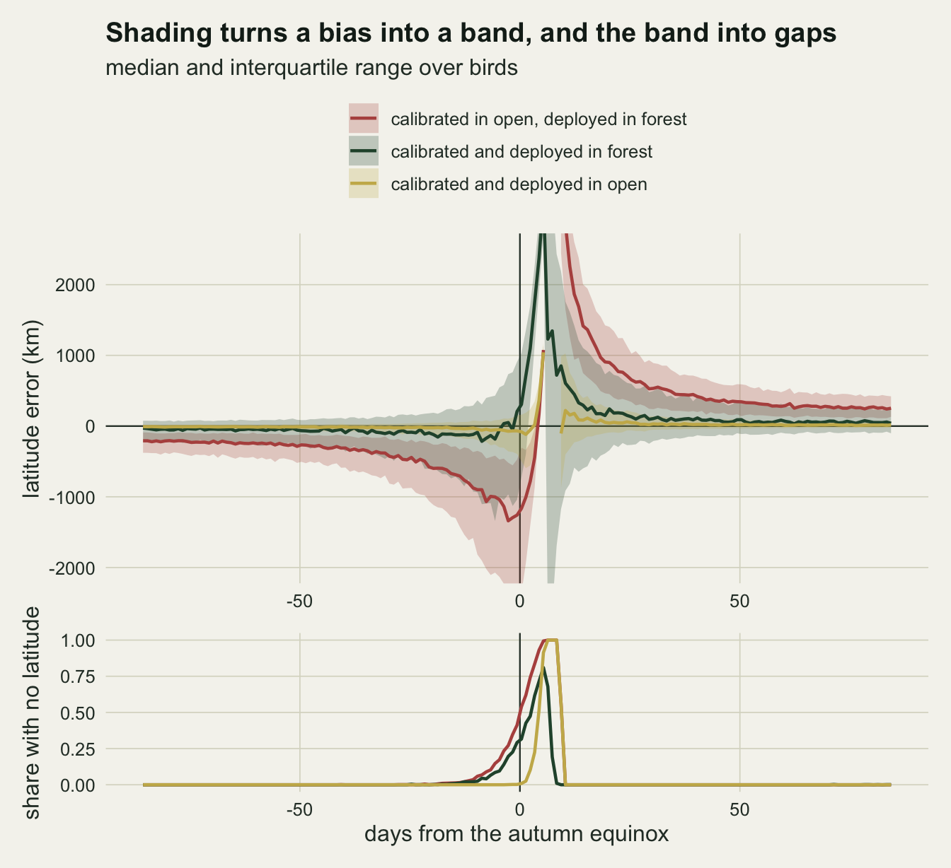
How wide the excluded window has to be
A common rule is to drop a fixed number of days either side of the equinox, often two to three weeks. The chunk below asks the question the other way round. For each day, take the median absolute latitude error over 1000 birds, counting a day with no latitude as a failure, and call the day usable when that median is below 200 km. The window edge on each side is the furthest day from the equinox that is not usable. Calibration is either in the open (mean shading 0.5 degrees) or in the deployment habitat, and deployment shading runs from a mean of 0.5 to 3 degrees.
limit_km <- 200
window_edges <- function(err) {
  abs_err <- abs(err); abs_err[is.na(abs_err)] <- Inf
  fails <- apply(abs_err, 2, median) >= limit_km
  pre  <- if (any(fails & day_eq < 0)) max(-day_eq[fails & day_eq < 0]) else 0
  post <- if (any(fails & day_eq > 0)) max(day_eq[fails & day_eq > 0]) else 0
  c(pre = pre, post = post)
}
usable_days <- function(err) {
  abs_err <- abs(err); abs_err[is.na(abs_err)] <- Inf
  ok <- apply(abs_err, 2, median) < limit_km
  c(pre = sum(ok & day_eq < 0), post = sum(ok & day_eq > 0))
}
dep_levels <- c(0.5, 1, 1.5, 2, 3)
set.seed(2004)
win_tab <- do.call(rbind, lapply(dep_levels, function(ds) {
  open_run <- run_scenario(0.5, ds)
  same_run <- run_scenario(ds, ds)
  rbind(data.frame(calibration = "open (mean 0.5)", dep_shade = ds, side = c("before", "after"),
                   edge = window_edges(open_run$err), usable = usable_days(open_run$err)),
        data.frame(calibration = "same habitat", dep_shade = ds, side = c("before", "after"),
                   edge = window_edges(same_run$err), usable = usable_days(same_run$err)))
}))
cap_before <- max(-day_eq)
cap_after  <- max(day_eq)
use_of <- function(cal, ds, sd_) win_tab$usable[win_tab$calibration == cal & win_tab$dep_shade == ds & win_tab$side == sd_]
win_of <- function(cal, ds, sd_) win_tab$edge[win_tab$calibration == cal & win_tab$dep_shade == ds & win_tab$side == sd_]
The simulated season reaches 86 days before the equinox and 84 days after it, so an edge at those values means no day on that side was usable. With both calibration and deployment in the open, the window runs from 2 days before the equinox to 17 days after it, lopsided because the blind day falls after the equinox. An open calibration with forest shading of mean 1 degree pushes the edges to 20 and 31 days, mean 1.5 to 49 and 65 days, and at mean 2 the furthest failing day is the first day of the season before the equinox and the last day after it. That does not mean every day fails: the same run has 1 usable day before the equinox and 0 after it. Calibrating in the same habitat gives 14 and 27 days at mean 1, 37 and 53 days at mean 2, and 75 and 84 days at mean 3, where no day after the equinox is usable. A matched calibration keeps the window inside the season up to a mean of 2 degrees, but at that shading it is already wider than the customary three weeks: the per-day noise, which no calibration removes, is enlarged near the equinox by the same geometry that enlarges the bias.
win_plot <- win_tab
cap_df <- data.frame(side = factor(c("before the equinox", "after the equinox"),
                                   levels = c("before the equinox", "after the equinox")),
                     cap = c(cap_before, cap_after))
win_plot$side <- factor(win_plot$side, levels = c("before", "after"),
                        labels = c("before the equinox", "after the equinox"))
ggplot(win_plot, aes(dep_shade, edge, colour = calibration, shape = calibration)) +
  geom_hline(data = cap_df, aes(yintercept = cap), colour = te_body, linetype = "dashed",
             linewidth = 0.5) +
  geom_hline(yintercept = 21, colour = te_line, linewidth = 1.2) +
  geom_line(linewidth = 0.8) +
  geom_point(size = 2.8) +
  facet_wrap(~ side) +
  scale_colour_manual(values = c("open (mean 0.5)" = te_rust, "same habitat" = te_forest),
                      name = "calibration") +
  scale_shape_manual(values = c("open (mean 0.5)" = 16, "same habitat" = 17),
                     name = "calibration") +
  scale_x_continuous(breaks = dep_levels) +
  labs(x = "mean deployment shading (degrees of elevation)",
       y = "window edge (days from equinox)",
       title = "The excluded window grows with shading",
       subtitle = "pale line: three weeks; dashed line: end of the simulated season") +
  theme_datasheet() +
  theme(legend.position = "bottom")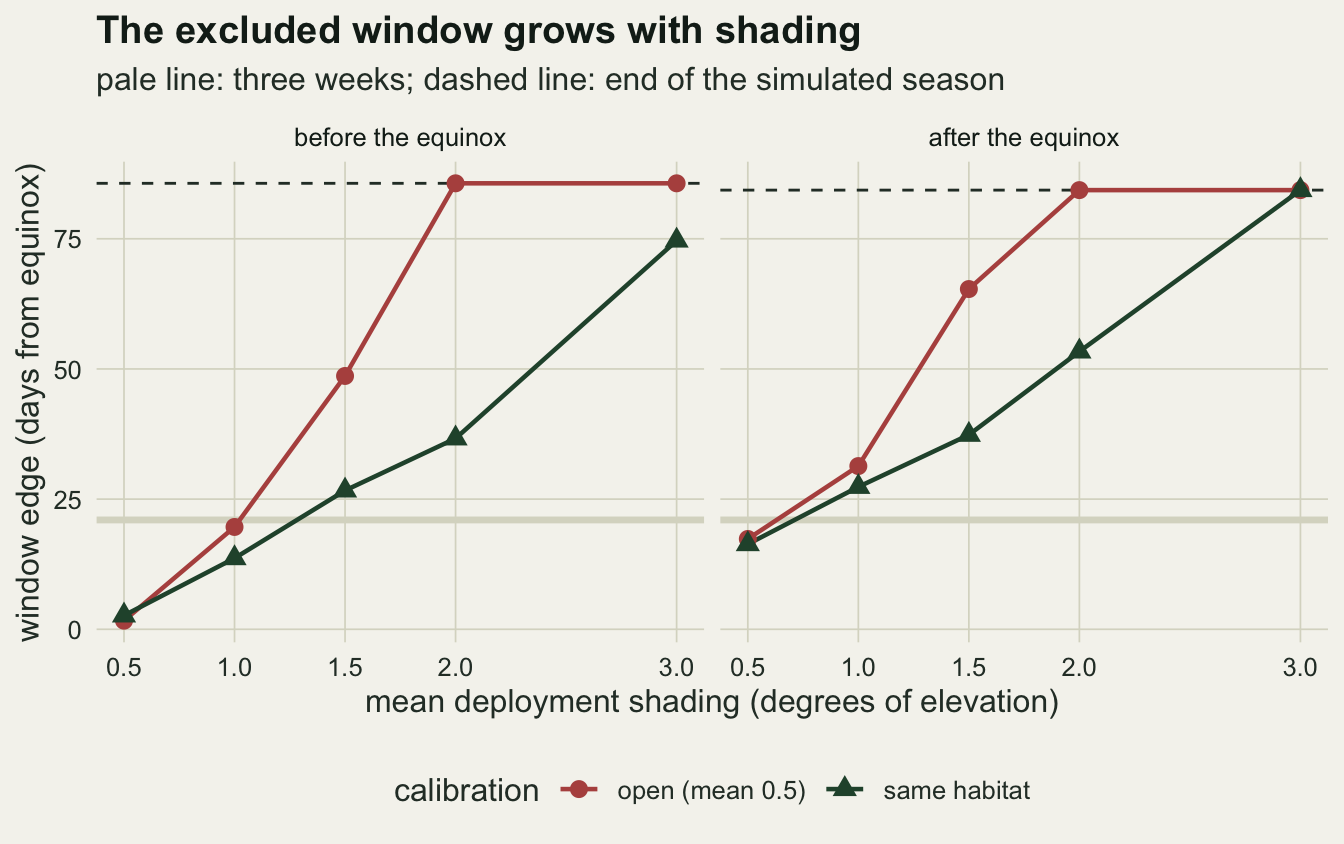
Shading as a delay at dawn
Exponential shading in elevation units, independent at both ends of the day, is one model. A bird that roosts in a cavity or dense cover and emerges after sunrise produces something else: a morning delay in time, with the evening unaffected. The chunk below keeps open-habitat shading at both twilights and adds a dawn delay in minutes, exponential with a mean chosen so that the average daylength lost equals the extra loss from forest shading (mean 2 instead of 0.5 degrees) beyond three weeks from the equinox. That mean is computed, not tuned. Calibration is in the open.
set.seed(1994)
loss_min <- function(shade_mean, n = 4000) {
  keep <- abs(day_eq) > 21
  h_clean <- hour_angle(lat_home, declination(days[keep]), elev_true)
  sim <- simulate_half_days(days[keep], shade_mean, n)
  mean(sweep(-sim$half, 2, h_clean, "+"), na.rm = TRUE) * 2 * 1440 / (2 * pi)
}
extra_loss <- loss_min(2) - loss_min(0.5)
dawn_mean  <- extra_loss
a_cal_dawn <- calibrate(0.5, n_bird)
dawn_dep   <- simulate_half_days(days, 0.5, n_bird)
delay_rad  <- matrix(rexp(n_bird * length(days), 1 / dawn_mean), n_bird) * 2 * pi / 1440
dawn_fit   <- lat_roots(dawn_dep$half - delay_rad / 2, dawn_dep$decl,
                        matrix(a_cal_dawn, n_bird, length(days)))
dawn_err   <- matrix(km_deg * (dawn_fit$lat - lat_home), n_bird)
dawn_status <- matrix(dawn_fit$status, n_bird)
dawn_med_pre  <- median(dawn_err[, pre_far], na.rm = TRUE)
dawn_med_post <- median(dawn_err[, post_far], na.rm = TRUE)
dawn_fail_near <- mean(dawn_status[, near] != "one root")
dawn_fail_post <- mean(dawn_status[, post_3_14] != "one root")
dawn_edges <- window_edges(dawn_err)
The matched mean delay is 22.8 minutes. With the same average loss concentrated at dawn, the median error beyond three weeks is -246 km before the equinox and +336 km after it, against -277 and +349 km for shading split over both twilights. The share of bird-days with no latitude is 0.506 within three days of the equinox and 0.581 from 3 to 14 days after it, and the window edges are 69 and 84 days, against 86 and 84 days. Latitude sees only the total length of the day, so with matched loss the medians and failure shares change little. The window before the equinox is narrower under the dawn delay, because the edge at forest shading sits at the season limit and is sensitive to small changes in the daily median. The distinction matters for longitude, which a dawn-only delay shifts and a symmetric shading does not, and longitude is not simulated here.
Hill-Ekstrom calibration on a bird that did not move
Hill-Ekstrom calibration needs no calibration site. If the bird was stationary over a period spanning the equinox, the right angle is the one under which its latitude is flat, because a wrong angle tilts the track south on one side and north on the other. The published implementations (the Hill-Ekstrom calibration in GeoLight, and the zenith search in TwGeos, both described in the user’s guide by Lisovski et al. 2020) turn this into a single rule: choose the angle that minimises the standard deviation of latitude over the whole stationary period, with days that return no latitude left out. The chunk below does exactly that for 200 birds with forest shading (mean 2 degrees) that stay put from day 181 to day 351, searching a grid of angles from -8 to 1 in steps of 0.05.
Two further rules are run on the same simulated twilights for comparison, and neither is a published method. The first is the same standard deviation criterion computed only on days 14 to 36 either side of the equinox, the kind of window an analyst builds after dropping two weeks either side of the equinox. The second is the flattening condition itself, equal median latitudes before and after the equinox over the whole period. The estimated shift is the median latitude after the equinox minus the median before it, so a positive shift means the track moves north.
A second set of birds sits at 52 N before the equinox and at 49 N after it, a real move of 3 degrees south made at the equinox.
n_he <- 200
angle_grid <- seq(-8, 1, by = 0.05)
in_window <- abs(day_eq) >= 14 & abs(day_eq) <= 36
win_eq <- day_eq[in_window]
row_median <- function(m) apply(m, 1, median, na.rm = TRUE)
row_sd <- function(m) apply(m, 1, sd, na.rm = TRUE)
crit_names <- c("SD, whole season", "SD, days 14 to 36", "equal medians")
hill_ekstrom <- function(lat_track, shade_mean) {
  sim <- simulate_half_days(days, shade_mean, n_he, lat = lat_track)
  n_a <- length(angle_grid)
  crit  <- array(Inf, c(n_he, n_a, 3))
  shift <- array(NA, c(n_he, n_a, 3))
  gone  <- matrix(NA, n_he, n_a)
  for (k in seq_len(n_a)) {
    lat_k <- matrix(lat_north(sim$half, sim$decl, angle_grid[k]), n_he)
    lat_w <- lat_k[, in_window]
    shift_all <- row_median(lat_k[, day_eq > 0]) - row_median(lat_k[, day_eq < 0])
    shift_win <- row_median(lat_w[, win_eq > 0]) - row_median(lat_w[, win_eq < 0])
    crit[, k, 1] <- row_sd(lat_k)
    crit[, k, 2] <- row_sd(lat_w)
    crit[, k, 3] <- abs(shift_all)
    shift[, k, 1] <- shift_all
    shift[, k, 2] <- shift_win
    shift[, k, 3] <- shift_all
    gone[, k] <- rowMeans(is.na(lat_k))
  }
  crit[is.na(crit)] <- Inf
  do.call(rbind, lapply(1:3, function(j) {
    pick <- apply(crit[, , j], 1, which.min)
    idx <- cbind(seq_len(n_he), pick)
    data.frame(criterion = crit_names[j], angle = angle_grid[pick],
               shift = shift[, , j][idx], missing = gone[idx])
  }))
}
set.seed(2020)
he_still <- hill_ekstrom(rep(lat_home, length(days)), 2)
move_deg <- 3
he_moved <- hill_ekstrom(ifelse(day_eq < 0, lat_home, lat_home - move_deg), 2)
he_light <- hill_ekstrom(rep(lat_home, length(days)), 1)
he_still$track <- "stationary at 52 N"
he_moved$track <- "moved 3 degrees south"
he_sum <- function(tab, crit, col, fun = mean) fun(tab[[col]][tab$criterion == crit])
se_mean <- function(v) sd(v) / sqrt(length(v))
share_below <- function(tab, crit) mean(tab$shift[tab$criterion == crit] < 0)
move_seen <- sapply(crit_names, function(cr)
  he_sum(he_moved, cr, "shift") - he_sum(he_still, cr, "shift"))
With the published rule, the stationary birds get a mean angle of -2.54 and a mean shift of +1.21 degrees (Monte Carlo standard error 0.14), northward although none of them moved. The shift varies a lot between birds: its standard deviation is 2.01 degrees, and 0.26 of the birds get a southward shift instead. At the chosen angle 0.036 of days return no latitude, so the criterion is not simply picking an angle that deletes the awkward days. The flattening condition picks -2.29 on average and, by construction, a shift of 0.00. The smallest spread of latitude and the flattest track are reached at different angles.
Restricting the same criterion to days 14 to 36 moves the mean angle to -2.13 and reverses the mean shift to -1.28 degrees (standard error 0.16). Taking out the days closest to the equinox, where a wrong angle distorts latitude most, changes which way the error goes. With lighter shading, mean 1 degree, the whole-season shift is +0.38 and the windowed one -0.90 degrees: smaller, with the same pattern of signs. In these runs the sign of the spurious shift was set by which days enter the criterion and its size grew with shading, so neither is something a reader can correct for after the fact.
The moved birds show what the calibration does to a real change of latitude. Their true shift is -3 degrees. The published rule estimates -0.64 on average, which is -1.85 degrees away from what it gave the stationary birds; the windowed rule -1.68, only -0.40 away from its stationary value; and the flattening condition +0.01, which erases the move completely because a flat track is what it asks for. The difference went into the angle: under the published rule it went from -2.54 to -2.77. That is the assumption of the method stated as a result: a bird that moves across the equinox breaks Hill-Ekstrom calibration, part of the move is turned into a change of angle, and nothing in the calibrated track says how much.
he_plot <- rbind(he_still, he_moved)
he_plot$track <- factor(he_plot$track, levels = c("stationary at 52 N", "moved 3 degrees south"))
he_plot$criterion <- factor(he_plot$criterion, levels = crit_names)
true_shift <- data.frame(track = factor(levels(he_plot$track), levels = levels(he_plot$track)),
                         truth = c(0, -move_deg))
he_means <- aggregate(shift ~ track + criterion, data = he_plot, FUN = mean)
ggplot(he_plot, aes(criterion, shift, colour = criterion)) +
  geom_hline(data = true_shift, aes(yintercept = truth), colour = te_ink,
             linetype = "dashed", linewidth = 0.6) +
  geom_jitter(width = 0.22, height = 0, alpha = 0.35, size = 1.2) +
  geom_point(data = he_means, shape = 23, size = 3.6, fill = te_paper, stroke = 1.2) +
  facet_wrap(~ track) +
  scale_colour_manual(values = setNames(c(te_rust, te_forest, te_gold), crit_names),
                      guide = "none") +
  scale_x_discrete(labels = c("SD\nwhole season", "SD\ndays 14 to 36", "equal\nmedians")) +
  coord_cartesian(ylim = c(-9.5, 11)) +
  labs(x = "criterion minimised", y = "estimated shift (degrees, north positive)",
       title = "The calibration invents one shift and shrinks another",
       subtitle = "forest shading, mean 2 degrees; days 181 to 351") +
  theme_datasheet()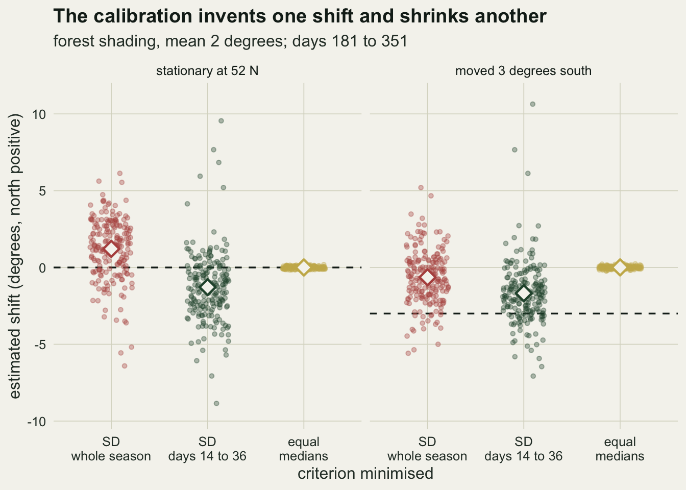
What to report
Report the sun elevation angle, how it was calibrated, and where. An angle taken from a logger in the open and applied to a forest bird moved the median latitude by -277 km before the equinox and +349 km after it in this simulation, which is a systematic error no amount of averaging across days removes. A reader cannot judge a latitude without that sentence.
State the excluded window in days before and after the equinox separately, and justify it. The blind day for a threshold angle below the horizon lies after the autumn equinox (here 8.1 days for an angle of -4 at 52 N, and later for lower angles) and before the spring one, so a symmetric window protects the wrong side. A window of three weeks was not enough for forest shading of mean 2 degrees even with a matched calibration.
Report how many days produced no latitude and whether that was because no latitude fits or because two do. Discarded days near the equinox are not missing at random; they are the days on which the bird’s track is least known.
If Hill-Ekstrom calibration was used, report the criterion, the days it was computed on, and the evidence that the bird was stationary. Under the conditions here the published rule gave a stationary bird a mean shift of +1.21 degrees, the same rule on a window without the equinox days -1.28 degrees, and a real move of 3 degrees survived at best as a change of 1.85 degrees. A latitude change across the equinox that is smaller than the between-bird spread of the spurious shift (2.01 degrees here) should not be read as movement.
Honest limits
The threshold method is the simplest analysis and no longer the usual one. Template-fit and state-space approaches (FLightR, SGAT and relatives, described in the user’s guide by Lisovski et al. 2020) use the whole light curve and a movement model, and they deal with the equinox by carrying the uncertainty rather than dropping days. The geometry that makes the threshold latitude fail is still the geometry those methods face, but the size of the errors and windows measured here does not carry over to them.
The shading model is exponential and independent between twilights and between days. Real shading is often autocorrelated: a bird that roosts in the same thicket for a week shades every twilight similarly, which moves part of the noise into a bias that changes with roost. Cloud adds shading that is shared by all birds on a day. Neither was simulated, and both would change the failure shares and the window. Only one latitude (52 N) and one base angle (-4) were used; the blind day moves with both, so the windows here belong to this design. The shading is modelled in elevation units, while state-space methods such as SGAT describe twilight error in minutes on both sides of the day; the dawn-only variant above is one time-unit model, not that one.
Unsolvable days were defined for an analyst who knows the hemisphere and accepts no ambiguity. An analyst who restricts latitude to a plausible band, say 40 to 60 N, would resolve some of the two-root days and would report fewer failures, at the price of placing some of them at the edge of the band.
The Hill-Ekstrom implementation is a grid search that follows the published rule (smallest standard deviation of latitude, days without a latitude left out) but is not the GeoLight or TwGeos code, and it works on simulated twilights without the outlier filtering that real data get first. The windowed standard deviation and the equal-medians condition are comparisons constructed for this post, not published methods. Only two window choices and two shading levels were run; they are enough to show that the sign of the spurious shift depends on the design, not to map that dependence. Lisovski et al. (2012) compared calibration methods on stationary loggers and found that calibration can shift estimated latitudes; whether they report this particular pre and post equinox artefact was not checked against the full text, so the post does not attribute it to them.
The birds here are stationary or make a single step. Longitude, which a geolocator estimates better than latitude, is ignored, and so is the refinement of positions by a movement model or a land mask, which in practice removes some of the worst latitudes near the equinox.
References
Hill RD 1994 In Le Boeuf BJ, Laws RM (eds) Elephant Seals, University of California Press, pp 227-236 (ISBN 0-520-08364-4)
Lisovski S, Hewson CM, Klaassen RHG, Korner-Nievergelt F, Kristensen MW, Hahn S 2012 Methods in Ecology and Evolution 3(3):603-612 (10.1111/j.2041-210X.2012.00185.x)
Ekstrom PA 2004 Memoirs of National Institute of Polar Research Special Issue 58:210-226
Lisovski S, Bauer S, Briedis M, Davidson SC, Dhanjal-Adams KL, Hallworth MT, Karagicheva J, Meier CM, Merkel B, Ouwehand J, Pedersen L, Rakhimberdiev E, Roberto-Charron A, Seavy NE, Sumner MD, Taylor CM, Wotherspoon SJ, Bridge ES 2020 Journal of Animal Ecology 89(1):221-236 (10.1111/1365-2656.13036)
Fudickar AM, Wikelski M, Partecke J 2012 Methods in Ecology and Evolution 3(1):47-52 (10.1111/j.2041-210X.2011.00136.x)
Forsythe WC, Rykiel EJ, Stahl RS, Wu H, Schoolfield RM 1995 Ecological Modelling 80(1):87-95 (10.1016/0304-3800(94)00034-F)