library(ggplot2)
library(survival)
library(patchwork)

te_paper  <- "#f5f4ee"
te_ink    <- "#16241d"
te_body   <- "#2c3a31"
te_forest <- "#275139"
te_rust   <- "#b5534e"
te_gold   <- "#c9b458"
te_line   <- "#dad9ca"

theme_datasheet <- function() {
  theme_minimal(base_size = 12) +
    theme(plot.background  = element_rect(fill = te_paper, colour = NA),
          panel.background = element_rect(fill = te_paper, colour = NA),
          panel.grid.major = element_line(colour = te_line, linewidth = 0.3),
          panel.grid.minor = element_blank(),
          text             = element_text(colour = te_body),
          plot.title       = element_text(colour = te_ink, face = "bold"),
          plot.subtitle    = element_text(colour = te_body),
          axis.text        = element_text(colour = te_body),
          strip.text       = element_text(colour = te_ink))
}Fire return intervals from a short scar record
R
fire ecology
survival analysis
simulation
ecology tutorial
With random fires, a mean fire interval from a short fire-scar record runs short, censoring both open gaps overshoots, and fire counts err less. Tested in R.
A pine stand on a dry ridge carries its fire history in its trunks. Low surface fires burn the base of the stem, the cambium heals around the wound, and a core or a wedge cut from the scarred face gives the calendar year of each fire to the ring. A fire historian who crossdates one well scarred tree might find four fires between 1850 and 1950. The number that goes into the report and the management plan is the mean fire interval: the mean of the gaps between consecutive scars. With four fires there are three gaps, and the open stretches before the first scar and after the last one are left out because nobody knows how long they were.
Johnson and Gutsell’s 1994 review of fire frequency models and methods is the standard account of how such intervals should be estimated, and Baker and Ehle argued in 2001 that intervals in ponderosa pine forests had been reported too short, partly because the gap between tree origin and the first scar is dropped. Grissino-Mayer fitted Weibull distributions to fire interval data from the American Southwest and read summary intervals off the fitted curve. None of what follows is a new finding; it is a measurement of those arguments on simulated records whose true mean interval is known, so the size of each bias can be put next to the length of the record and the regularity of the fires.
This site has three posts on censored durations, and the fire record looks like their subject until the details are read. Kaplan-Meier survival curves and the log-rank test censors collared animals that are still alive when the study ends. Parametric survival and the AFT model fits a Weibull with survreg and reads it as a hazard model and a time model at once. Interval-censored survival from visit data shows how coding the deaths in the interval before the first check at its midpoint distorts the fitted shape. In all three every animal is a separate unit with its own clock starting at a known time. A scar record is one sequence of events from a renewal process, and the observation window cuts it at both ends. The reflex those posts teach, give every incomplete record a censoring type instead of dropping it, turns out to be the wrong repair for one of the two ends, and on a record four mean intervals long the plainest estimator of all does better than that reflex.
The post measures four things: the arithmetic of the naive mean when fires arrive at random, how that bias depends on the regularity of the fire regime and on the usual rule that a record needs at least three fires, what the censored Weibull does with each end of the record, and what happens when several trees are pooled into a composite record.
Six estimators for one record
Fires at one point follow a stationary renewal process: the gaps between fires are independent Weibull draws with a mean of 25 years and a shape of 1, 2 or 3. Shape 1 is the exponential, fires with no memory of the last one. Shape 3 is a regime in which fuel has to build up before the next fire can carry, so gaps cluster around the mean. Each process runs for 2000 years before the record opens, so the record starts at a time unrelated to any fire. Records last 2, 4 or 8 mean intervals, which is 50, 100 or 200 years. These design constants, and the 1000 records per cell, were fixed before the first run.
Every record is summarised six ways. The naive mean fire interval is the mean of the complete gaps between the first and last scar. The Weibull median probability interval is the median of a two-parameter Weibull fitted to those complete gaps, a summary that fire history software reports; Grissino-Mayer fitted such distributions and preferred the modal interval, but the selection problem is the same for either. It estimates the median of the interval distribution, not the mean, so it is scored against the true median. The censored Weibull with both ends keeps the gap from the record start to the first fire and the gap from the last fire to the record end as right-censored observations, which is what a survival analyst would do first. The censored Weibull with the end gap only drops the first gap. The stationary likelihood treats the first gap as what it is under a renewal process that started long before the record, a forward recurrence time, whose density is the Weibull survival function divided by the mean. The count estimator is the record length divided by the number of fires.
mu_true  <- 25
run_in   <- 2000
shapes   <- c(1, 2, 3)
len_mult <- c(2, 4, 8)
n_rep    <- 1000
min_fire <- 3

sim_records <- function(n_rec, shape, rec_len) {
  scale_w <- mu_true / gamma(1 + 1 / shape)
  n_int   <- ceiling((run_in + rec_len) / mu_true * 1.6 + 40)
  gaps    <- matrix(scale_w * rweibull(n_rec * n_int, shape), n_rec)
  fire_t  <- t(apply(gaps, 1, cumsum)) - run_in
  stopifnot(all(fire_t[, n_int] > rec_len))
  lapply(seq_len(n_rec), function(i) {
    x_i <- fire_t[i, ]
    x_i[x_i > 0 & x_i <= rec_len]
  })
}

weib_profile <- function(events, censored) {
  n_ev   <- length(events)
  all_t  <- c(events, censored)
  sum_lg <- sum(log(events))
  prof_ll <- function(log_k) {
    k_w <- exp(log_k)
    n_ev * log_k - n_ev * log(sum(all_t^k_w) / n_ev) + (k_w - 1) * sum_lg - n_ev
  }
  opt     <- optimize(prof_ll, c(-4, 4), maximum = TRUE)
  k_w     <- exp(opt$maximum)
  scale_w <- (sum(all_t^k_w) / n_ev)^(1 / k_w)
  c(shape = k_w, scale = scale_w, edge = sign(opt$maximum) * (abs(opt$maximum) > 3.99))
}

weib_stationary <- function(intervals, gap_first, gap_last, start) {
  neg_ll <- function(par) {
    k_w <- exp(par[1])
    scale_w <- exp(par[2])
    mean_w <- scale_w * gamma(1 + 1 / k_w)
    -(sum(dweibull(intervals, k_w, scale_w, log = TRUE)) +
        pweibull(gap_last, k_w, scale_w, lower.tail = FALSE, log.p = TRUE) +
        pweibull(gap_first, k_w, scale_w, lower.tail = FALSE, log.p = TRUE) -
        log(mean_w))
  }
  opt <- optim(start, neg_ll, control = list(maxit = 1000))
  c(shape = exp(opt$par[1]), scale = exp(opt$par[2]), code = opt$convergence)
}

estimate_record <- function(x_f, rec_len) {
  n_f     <- length(x_f)
  iv      <- diff(x_f)
  g_first <- x_f[1]
  g_last  <- rec_len - x_f[n_f]
  f_both  <- weib_profile(iv, c(g_first, g_last))
  f_end   <- weib_profile(iv, g_last)
  f_iv    <- weib_profile(iv, numeric(0))
  f_stat  <- weib_stationary(iv, g_first, g_last,
                             c(log(max(f_both[1], 0.05)), log(f_both[2])))
  wmean <- function(f) unname(f[2] * gamma(1 + 1 / f[1]))
  c(n_fire = n_f, naive = mean(iv),
    wmpi = unname(f_iv[2] * log(2)^(1 / f_iv[1])),
    cens_both = wmean(f_both), cens_end = wmean(f_end),
    stationary = wmean(f_stat), count = rec_len / n_f,
    edge_both = unname(f_both[3]), edge_end = unname(f_end[3]),
    code_stat = unname(f_stat[3]))
}
The Weibull fits use the profile likelihood: for a fixed shape the maximum likelihood scale has a closed form, so only the shape needs a one-dimensional search, bounded between exp(-4) and exp(4). The stationary likelihood has no such shortcut and is maximised with optim() from the censored fit’s estimate. Records with fewer than three fires are set aside before any estimator is computed, which is a common minimum in fire history summaries, and the share set aside is reported with every result because the rule is part of the estimator.
set.seed(1998)
cells <- expand.grid(shape = shapes, len_mult = len_mult)
sim_out <- lapply(seq_len(nrow(cells)), function(i) {
  rec_len <- cells$len_mult[i] * mu_true
  recs <- sim_records(n_rep, cells$shape[i], rec_len)
  n_f  <- lengths(recs)
  ok   <- n_f >= min_fire
  est  <- t(vapply(recs[ok], estimate_record, numeric(10), rec_len = rec_len))
  list(n_fire = n_f, est = est, recs = recs[ok], rec_len = rec_len)
})

est_names <- c("naive", "cens_both", "cens_end", "stationary", "count")
summ <- do.call(rbind, lapply(seq_len(nrow(cells)), function(i) {
  est_i <- sim_out[[i]]$est
  med_true <- mu_true / gamma(1 + 1 / cells$shape[i]) * log(2)^(1 / cells$shape[i])
  rbind(
    data.frame(shape = cells$shape[i], len_mult = cells$len_mult[i],
               estimator = est_names,
               med = apply(est_i[, est_names], 2, median) / mu_true,
               avg = colMeans(est_i[, est_names]) / mu_true,
               rmse = sqrt(colMeans((est_i[, est_names] / mu_true - 1)^2)),
               short = mean(sim_out[[i]]$n_fire < min_fire), kept = nrow(est_i)),
    data.frame(shape = cells$shape[i], len_mult = cells$len_mult[i],
               estimator = "wmpi",
               med = median(est_i[, "wmpi"]) / med_true,
               avg = mean(est_i[, "wmpi"]) / med_true,
               rmse = sqrt(mean((est_i[, "wmpi"] / med_true - 1)^2)),
               short = mean(sim_out[[i]]$n_fire < min_fire), kept = nrow(est_i)))
}))
rownames(summ) <- NULL
pick <- function(est, shp, lm, col) {
  summ[summ$estimator == est & summ$shape == shp & summ$len_mult == lm, col]
}
rmse_of <- function(est) summ$rmse[summ$estimator == est & summ$len_mult >= 4]
stat_count_gap <- max(abs(rmse_of("stationary") - rmse_of("count")))
edge_share <- max(vapply(sim_out, function(s) mean(s$est[, "edge_both"] != 0), 0))
edge_lower <- sum(vapply(sim_out, function(s) sum(s$est[, c("edge_both", "edge_end")] < 0), 0))
edge_upper <- sum(vapply(sim_out, function(s) sum(s$est[, c("edge_both", "edge_end")] > 0), 0))
med_nfire <- median(sim_out[[4]]$est[, "n_fire"])
stat_codes <- sum(vapply(sim_out, function(s) sum(s$est[, "code_stat"] != 0), 0))
When fires are random the bias is arithmetic
For shape 1 the fires form a Poisson process, and given n fires in a record of length L their dates are n uniform order statistics. The n fires cut the record into n + 1 exchangeable pieces, each with expectation L/(n + 1). The naive mean spans n - 1 of those pieces and divides by n - 1, so its expectation given n is L/(n + 1). The count estimator is L/n. An exponential fit with both open gaps censored has a total exposure of L and n - 1 events, so its estimate is L/(n - 1). Three estimators of the same interval differ only in their denominator, and the number of fires is Poisson with mean L/mu. Averaging over n, conditional on at least three fires, gives exact expectations.
exact_ratio <- function(lm) {
  n_all <- 0:400
  p_all <- dpois(n_all, lm)
  keep  <- n_all >= min_fire
  w_n   <- p_all[keep] / sum(p_all[keep])
  n_k   <- n_all[keep]
  c(short = 1 - sum(p_all[keep]),
    naive = sum(w_n * lm / (n_k + 1)),
    count = sum(w_n * lm / n_k),
    expo_both = sum(w_n * lm / (n_k - 1)))
}
exact_tab <- sapply(len_mult, exact_ratio)
colnames(exact_tab) <- len_mult
ex4 <- exact_tab[, "4"]
cv2 <- gamma(1 + 2 / shapes) / gamma(1 + 1 / shapes)^2 - 1
mc_se_naive <- sd(sim_out[[4]]$est[, "naive"] / mu_true) / sqrt(nrow(sim_out[[4]]$est))
gap_naive_se <- abs(pick("naive", 1, 4, "avg") - ex4["naive"]) / mc_se_naive
At four mean intervals a record has fewer than three fires with probability 0.238, and among the rest the exact expected ratios to the true mean are 0.744 for the naive mean, 0.930 for the count and 1.257 for the exponential with both gaps censored. The simulated records agree: 0.235 set aside, and a mean naive ratio of 0.728, 1.4 Monte Carlo standard errors from the exact value. At two mean intervals the exact figures are 0.677 set aside and 0.442, 0.573 and 0.819 for the three estimators; at eight they are 0.014, 0.971, 1.126 and 1.355.
Two things in those numbers are not about the naive mean. The count estimator is below one at two and four mean intervals although the number of fires in a stationary record has expectation exactly L/mu. The three fire rule removes the records with the fewest fires, which are the records whose count estimate would have been largest, and at two mean intervals it removes most of them. At eight mean intervals almost nothing is removed and the count estimate sits above one instead, because the mean of L/n is larger than L divided by the mean of n. The rule and the reciprocal pull in opposite directions, and which one wins depends on how often the rule bites.
Regular fire hides the truncation
The arithmetic above is special to shape 1. When fire needs fuel to recover, gap lengths vary less, and an interval that straddles the record boundary is less exaggerated than a typical one. Under a stationary renewal process its expected length is the mean times one plus the squared coefficient of variation of the gaps: 2.00 times the mean at shape 1 but only 1.27 times at shape 2 and 1.13 at shape 3. The gaps a window loses at its ends are still longer than the ones it keeps, only by less. The simulation measures how much of the bias survives.
naive_s <- summ[summ$estimator == "naive", ]
short_answer <- mean(sim_out[[4]]$est[, "naive"] < mu_true)
wmpi_s  <- summ[summ$estimator == "wmpi", ]
At four mean intervals the naive mean has a median ratio of 0.672 at shape 1, 0.883 at shape 2 and 0.964 at shape 3, and mean ratios of 0.728, 0.924 and 0.995. The mean sits closer to one than the median at shape 1 because the naive mean is itself right skewed, and the mean alone would hide that 0.821 of the retained shape 1 records give an answer below the true mean. At shape 3 both are within 4 per cent of the truth.
At two mean intervals the three fire rule changes which records are analysed at all. It sets aside 0.673 of shape 1 records and 0.793 of shape 3 records, because a regular regime rarely fits three fires into two mean intervals. The records that survive are the ones with fires packed close together, and the naive median ratio is 0.411, 0.631 and 0.711 at the three shapes. With three fires in two mean intervals the two complete gaps cannot sum to more than the record, so the naive mean cannot exceed the true mean at all. Regularity does not rescue a record that was only kept because it happened to be short.
The Weibull median probability interval fitted to the complete gaps inherits the same selection. Scored against the true median of the interval distribution, its median ratio at four mean intervals is 0.789 at shape 1 and 0.973 at shape 3, and at two mean intervals 0.476 and 0.705. Fitting a distribution to the gaps changes the summary, not the data it summarises.
naive_long <- rbind(
  data.frame(naive_s[, c("shape", "len_mult")], value = naive_s$med, stat = "median"),
  data.frame(naive_s[, c("shape", "len_mult")], value = naive_s$avg, stat = "mean"))
naive_long$shape <- factor(paste("shape", naive_long$shape))
short_df <- naive_s
short_df$shape <- factor(paste("shape", short_df$shape))
shape_cols <- c("shape 1" = te_rust, "shape 2" = te_gold, "shape 3" = te_forest)

p_bias <- ggplot(naive_long, aes(len_mult, value, colour = shape, linetype = stat)) +
  geom_hline(yintercept = 1, colour = te_body, linewidth = 0.4) +
  geom_line(linewidth = 0.8) +
  geom_point(size = 2.2) +
  scale_colour_manual(values = shape_cols, name = NULL) +
  scale_linetype_manual(values = c(median = "solid", mean = "dashed"), name = NULL) +
  scale_x_continuous(breaks = len_mult) +
  scale_y_continuous(limits = c(0.35, 1.05)) +
  labs(x = "record length (mean intervals)", y = "naive MFI / true mean",
       title = "Short records, short gaps")
p_short <- ggplot(short_df, aes(len_mult, short, colour = shape)) +
  geom_line(linewidth = 0.8) +
  geom_point(size = 2.2) +
  scale_colour_manual(values = shape_cols, name = NULL) +
  scale_x_continuous(breaks = len_mult) +
  scale_y_continuous(limits = c(0, 1)) +
  labs(x = "record length (mean intervals)", y = "share with fewer than 3 fires",
       title = "Records set aside")
(p_bias + p_short) +
  plot_layout(guides = "collect") +
  plot_annotation(theme = theme_datasheet()) &
  theme_datasheet() &
  theme(legend.position = "bottom")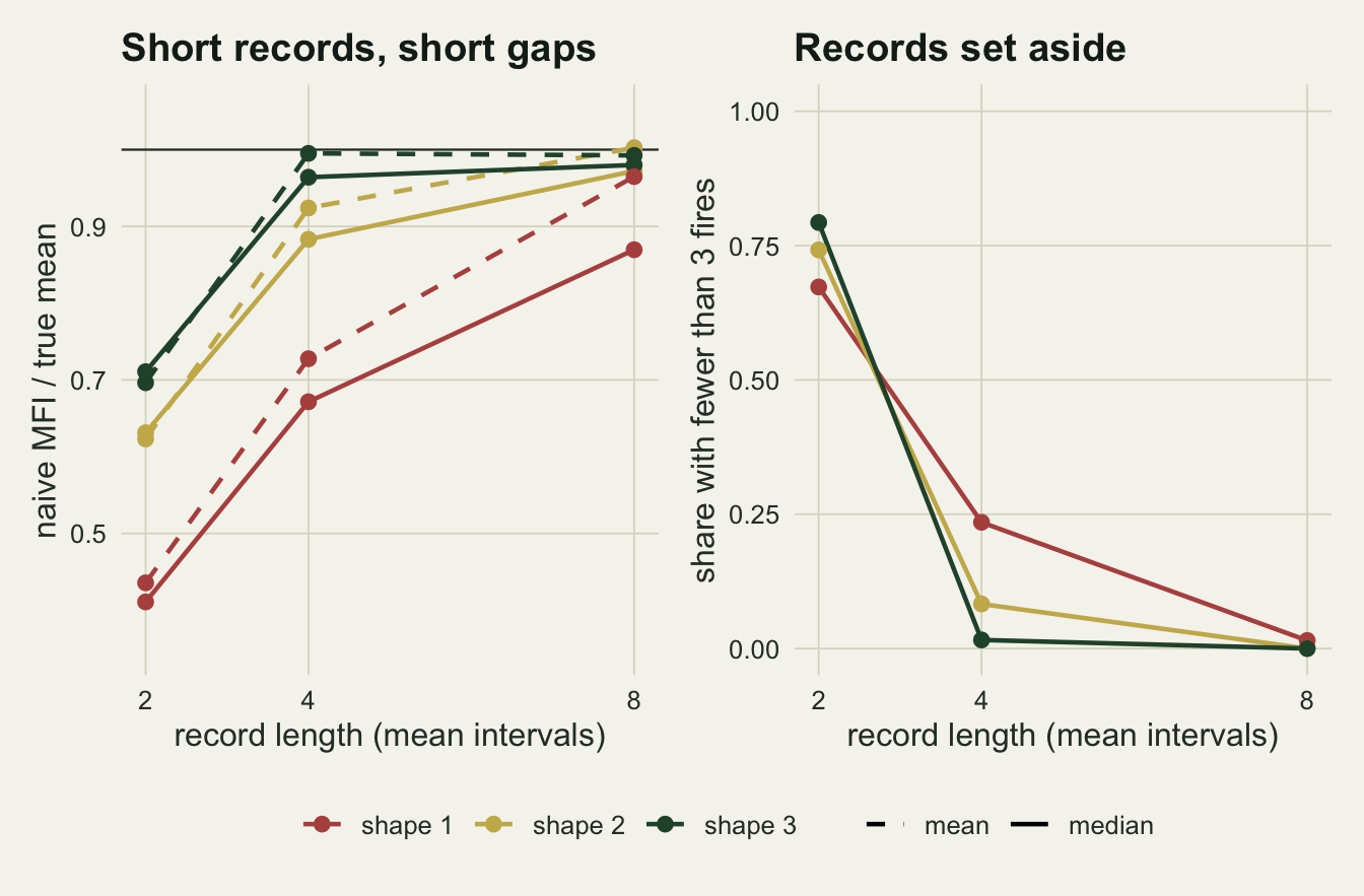
The survival reflex, and where the record starts
A reader of the survival posts would not drop the open gaps; they would censor them. The gap after the last scar is a textbook right-censored observation: a fire happened, and the next one had not happened by the time the tree was cut. Given the last fire, the waiting time to the next is a fresh draw from the interval distribution, and censoring it is correct. The gap before the first scar is different. The record did not open at a fire. It opened at some date, the pith of the tree or the start of the documentary record, that fell inside an interval already running. Under a stationary process that interval is length biased, because a long interval is more likely to contain an arbitrary date than a short one, and the distance from the date to the next fire has density S(t)/mu rather than f(t). Right censoring uses S(t) and ignores the 1/mu, so it tells the likelihood that the first gap was a normal interval of at least that length, which makes long intervals look more common than they are.
Which correction is right depends on where the record is taken to start, and that is the question a dendrochronologist asks first. If the record starts at the first scar, as it does when a tree becomes a recorder only once it has been wounded, then nothing before the first scar is data, and the likelihood conditional on the first fire is the complete gaps plus the censored end gap. If the record starts at a date unrelated to fire, the first gap is information, and it belongs in the likelihood as a forward recurrence time, or implicitly through the count estimator, which only needs that the record window is unrelated to the fires. Whether an inner ring is such a date is doubtful, and the honest limits come back to it.
reflex_s <- summ[summ$estimator %in% est_names & summ$len_mult == 4, ]

surv_check <- do.call(rbind, lapply(seq_len(nrow(cells)), function(i) {
  rec_len <- sim_out[[i]]$rec_len
  sr_fit <- vapply(sim_out[[i]]$recs, function(x_f) {
    n_f  <- length(x_f)
    tm   <- c(diff(x_f), x_f[1], rec_len - x_f[n_f])
    stat <- c(rep(1, n_f - 1), 0, 0)
    fit  <- suppressWarnings(survreg(Surv(tm, stat) ~ 1, dist = "weibull"))
    unname(c(exp(coef(fit)) * gamma(1 + fit$scale), fit$scale))
  }, numeric(2))
  sr_mean <- sr_fit[1, ]
  rel_gap <- abs(sr_mean / sim_out[[i]]$est[, "cens_both"] - 1)
  fin <- is.finite(sr_mean)
  data.frame(shape = cells$shape[i], n = length(rel_gap),
             agree = sum(fin & rel_gap < 0.01), nonfinite = sum(!fin),
             off = sum(fin & rel_gap >= 0.01), worst = max(sr_mean[fin]) / mu_true,
             collapse = sum((!fin | rel_gap >= 0.01) & sr_fit[2, ] < 0.001))
}))
sr_total <- sum(surv_check$n)
sr_agree <- sum(surv_check$agree)
sr_nonfin <- sum(surv_check$nonfinite)
sr_off <- sum(surv_check$off)
sr_worst <- max(surv_check$worst)
sr_collapse <- sum(surv_check$collapse)
sr_bad_regular <- sum(surv_check$nonfinite[surv_check$shape > 1] +
                        surv_check$off[surv_check$shape > 1])
The censored fits here were checked against survreg() on every retained record, 6443 fits with both open gaps censored: the two agree on the mean interval to within one per cent in 6417 of them. In 7 records survreg() returned a mean that was not a finite number, and in 19 more it returned a finite mean more than one per cent away, the largest 3.30e+26 times the true mean. 26 of those 26 disagreements came from shapes 2 and 3, and in 14 of the 26 the survreg() scale parameter, the reciprocal of the Weibull shape, had collapsed below a thousandth: nearly equal gaps with short censored ends let the fitted shape run off towards infinity. In such records the likelihood can keep rising with the shape, so there may be no maximum for either routine to find: the profile search then stops at its upper bound, and survreg() stops wherever its iterations end, so a disagreement there is not always an error of survreg() alone. A single such record is enough to make the average of the fitted means meaningless, so any summary over many censored fits needs these cases counted and reported. The profile search put the shape at one of its bounds in at most 0.0290 of records in any cell, 95 times at the upper bound and 0 times at the lower one across the both-gaps and end-gap fits, and optim() reported non-convergence of the stationary likelihood in 0 records.
At four mean intervals the censored Weibull with both gaps has a median ratio of 1.075, 1.038 and 1.040 at shapes 1, 2 and 3. It overshoots at every shape. At shape 1 its mean ratio is 1.405 and its root mean square error 1.956 of the true mean, because a record with few events and long censored gaps can pull the fitted shape well below one, and a Weibull mean grows very fast as the shape falls; the largest estimate among those 765 records was 27.2 times the true mean.
The two correctly specified likelihoods behave differently from each other. Conditioning on the first scar, the end gap only fit has a median of 0.877 and a mean of 1.019 at shape 1, with a root mean square error of 0.848: nearly unbiased on average but still exposed to fitted shapes well below one, which inflate a Weibull mean. The stationary likelihood, which uses the first gap properly, has a median of 0.923, a mean of 0.921 and a root mean square error of 0.293. The count estimator, which fits nothing, has a mean of 0.919 and a root mean square error of 0.287. Its median is exactly 1.000, which is less impressive than it looks: the count is an integer, and the median number of fires among the records kept is 4, so the median of the count estimate lands exactly on the true mean.
At shape 3 the differences almost vanish. The root mean square errors at four mean intervals are 0.215 for the naive mean, 0.215 with both gaps censored, 0.204 for the stationary likelihood and 0.211 for the count. Where fire is regular the choice of estimator is a matter of a few per cent; where fire is random it decides whether the answer is a third short, a few per cent long, or occasionally absurd.
est_lab <- c(naive = "naive MFI", cens_both = "censored, both gaps",
             cens_end = "censored, end gap", stationary = "stationary likelihood",
             count = "length / fires")
box_df <- do.call(rbind, lapply(which(cells$len_mult == 4), function(i) {
  est_i <- sim_out[[i]]$est[, est_names] / mu_true
  do.call(rbind, lapply(est_names, function(nm) {
    q_v <- quantile(est_i[, nm], c(0.05, 0.25, 0.5, 0.75, 0.95), names = FALSE)
    data.frame(shape = paste("shape", cells$shape[i]), estimator = est_lab[[nm]],
               q05 = q_v[1], q25 = q_v[2], q50 = q_v[3], q75 = q_v[4], q95 = q_v[5],
               avg = mean(est_i[, nm]))
  }))
}))
box_df$estimator <- factor(box_df$estimator, levels = rev(unname(est_lab)))

ggplot(box_df, aes(y = estimator)) +
  geom_vline(xintercept = 1, colour = te_body, linetype = "dashed", linewidth = 0.4) +
  geom_errorbar(aes(xmin = q05, xmax = q95), orientation = "y", width = 0,
                colour = te_body, linewidth = 0.5) +
  geom_crossbar(aes(x = q50, xmin = q25, xmax = q75), orientation = "y",
                fill = te_line, colour = te_forest, width = 0.55, linewidth = 0.4) +
  geom_point(aes(x = avg), shape = 23, size = 2.6, fill = te_rust, colour = te_ink) +
  facet_wrap(~ shape, ncol = 3) +
  scale_x_log10(breaks = c(0.25, 0.5, 1, 2, 4)) +
  labs(x = "estimate / true mean interval (log scale)", y = NULL,
       title = "Censoring both open gaps overshoots",
       subtitle = "records of 100 years, true mean interval 25 years") +
  theme_datasheet()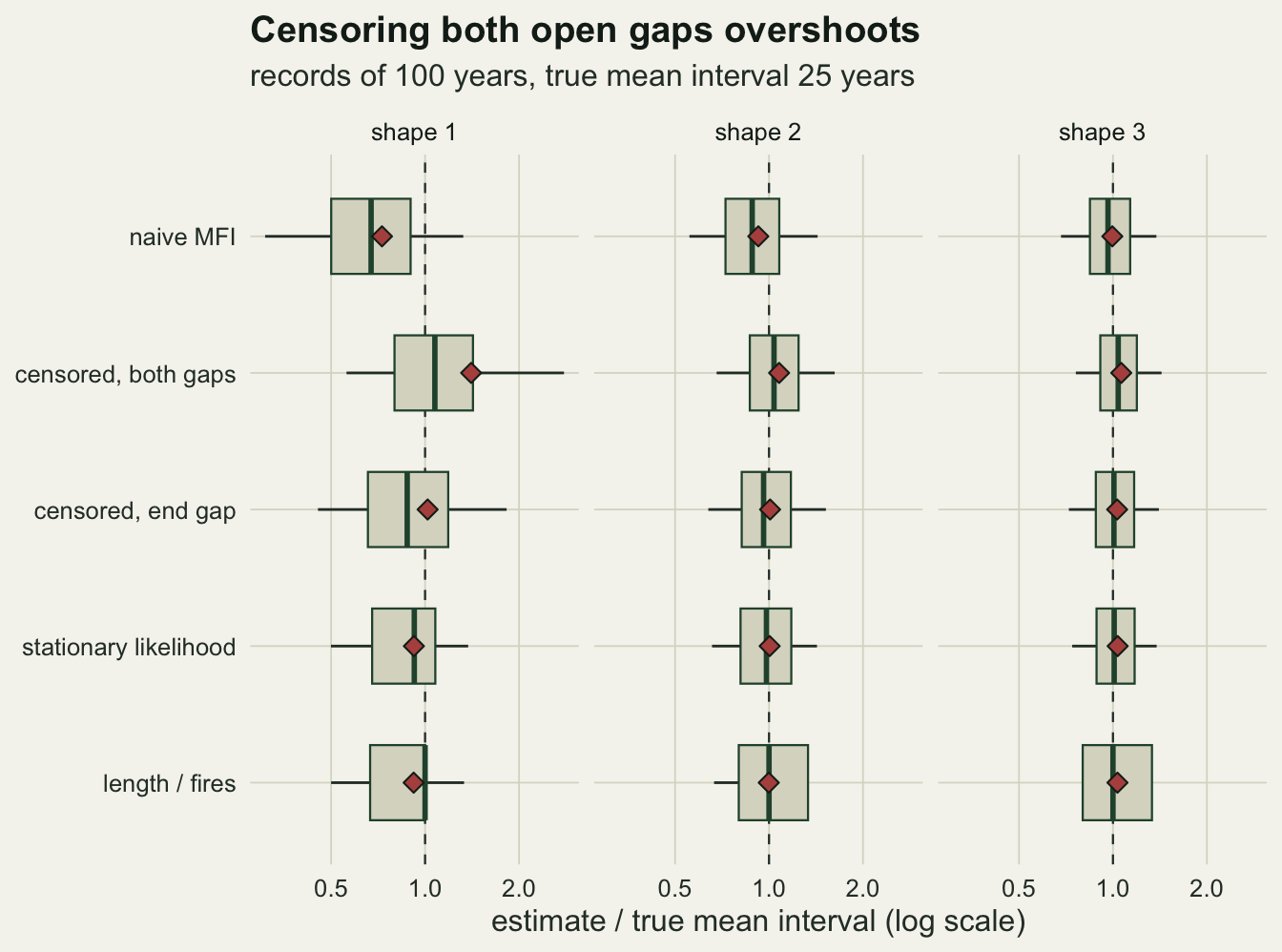
A composite of trees answers a different question
Fire historians rarely rely on one tree. Scar dates from many trees in a stand are pooled into a composite record, and because a single tree misses fires that did not reach it or did not wound it, the composite has more fires and shorter intervals. The composite interval therefore shrinks as more trees, or more ground, are added, and Baker and Ehle list the sampling of heavily scarred trees among the reasons reported intervals run short. Filters are the usual response. A fire is kept only if at least two trees recorded it, or at least two trees and at least ten per cent of the recording trees.
The simulation for this section is a separate design, fixed before it ran. Fires occur in the stand as a renewal process with a Weibull shape of 2 and a mean of 10 years. Each fire burns a random fraction of the stand drawn from a Beta(0.5, 1) distribution, so most fires are small, and each tree inside the burned fraction is scarred with probability 0.6. The record is 200 years long and there are 1000 simulated stands. Three reference intervals follow from those constants: every fire in the stand, every fire at a given point, and every scar on a given tree.
mu_area    <- 10
shape_area <- 2
comp_len   <- 200
comp_burn  <- 500
p_scar     <- 0.6
ext_a      <- 0.5
ext_b      <- 1
tree_grid  <- c(1, 2, 5, 10, 20, 40, 80)
n_comp     <- 1000
filters    <- c("any scar", "2 or more trees", "2 trees and 10 per cent")

mean_ext  <- ext_a / (ext_a + ext_b)
mu_point  <- mu_area / mean_ext
mu_tree   <- mu_point / p_scar
ext_cut   <- 0.1 / p_scar
keep_lim  <- pbeta(ext_cut, ext_a, ext_b, lower.tail = FALSE)
limit_ten <- mu_area / keep_lim / mu_point

one_stand <- function() {
  scale_a <- mu_area / gamma(1 + 1 / shape_area)
  n_draw  <- ceiling((comp_burn + comp_len) / mu_area * 1.5 + 30)
  fire_t  <- cumsum(scale_a * rweibull(n_draw, shape_area)) - comp_burn
  fire_t  <- fire_t[fire_t > 0 & fire_t <= comp_len]
  n_f     <- length(fire_t)
  extent  <- rbeta(n_f, ext_a, ext_b)
  scarred <- matrix(runif(n_f * max(tree_grid)) < extent * p_scar, n_f)
  cum_sc  <- matrix(t(apply(scarred, 1, cumsum)), n_f)
  out <- matrix(NA_real_, length(tree_grid) * 3, 3)
  row_i <- 0
  for (k_t in tree_grid) {
    need <- c(1, 2, max(2, ceiling(0.1 * k_t)))
    for (j in 1:3) {
      x_f <- fire_t[cum_sc[, k_t] >= need[j]]
      n_k <- length(x_f)
      row_i <- row_i + 1
      out[row_i, ] <- c(n_k,
                        if (n_k >= min_fire) mean(diff(x_f)) else NA,
                        if (n_k >= min_fire) comp_len / n_k else NA)
    }
  }
  out
}

set.seed(1983)
comp_arr <- replicate(n_comp, one_stand())
comp_s <- data.frame(trees = rep(tree_grid, each = 3),
                     filter = factor(rep(filters, length(tree_grid)), levels = filters))
comp_s$short <- apply(comp_arr[, 1, ], 1, function(v) mean(v < min_fire))
comp_s$naive <- apply(comp_arr[, 2, ], 1, mean, na.rm = TRUE) / mu_point
comp_s$count <- apply(comp_arr[, 3, ], 1, mean, na.rm = TRUE) / mu_point
comp_s$gap   <- abs(comp_s$naive / comp_s$count - 1)
cpick <- function(k_t, flt, col) comp_s[comp_s$trees == k_t & comp_s$filter == flt, col]
gap_many <- max(comp_s$gap[comp_s$trees >= 10], na.rm = TRUE)
With these constants the interval between fires anywhere in the stand is 10 years, the interval between fires at one point is 30 years, and the interval between scars on one tree is 50 years. The point interval is the quantity a fire return interval usually intends, so the results below are scaled by it.
A single tree gives a naive mean of 1.319 of the point interval: longer than the point interval because the tree misses fires, and shorter than the tree’s own scar interval, 1.667, because of the truncation measured above. An unfiltered composite falls to 0.639 at 5 trees, 0.446 at 20 and 0.382 at 80, heading for the stand interval at 0.333. The two tree filter slows the fall but does not stop it: 1.045, 0.534 and 0.411. The ten per cent filter almost levels off: 0.534 at 20 trees, 0.544 at 40 and 0.554 at 80.
The level it settles at is not the point interval, and it has a closed form. With many trees, a fire passes the ten per cent filter when the share of trees it scars, extent times 0.6, exceeds a tenth, which means an extent above 0.167. That happens to a share 0.592 of fires, so the filtered composite converges to the stand interval divided by that share, 0.563 of the point interval. The filter makes the composite depend only weakly on the number of trees, still rising slowly at 80 trees towards that limit; it does not make it estimate the interval at a point. What it estimates is set by the fire size distribution and the scarring probability, neither of which the scar record measures.
Against that, the choice between the naive mean and the count estimator nearly stops mattering. With 10 trees or more, in every filter, the two differ by at most 7 per cent, because a composite holds many fires and the ends of the record are a small part of it. Pooling trees fixes the truncation problem of the first sections and replaces it with a question about which fires count.
ref_df <- data.frame(y = c(mu_tree / mu_point, 1, limit_ten, mu_area / mu_point),
                     lab = c("one tree, all scars", "one point", "10 per cent filter limit",
                             "whole stand"))
filter_cols <- c("any scar" = te_rust, "2 or more trees" = te_gold,
                 "2 trees and 10 per cent" = te_forest)
comp_plot <- comp_s[is.finite(comp_s$naive), ]
comp_plot <- comp_plot[order(comp_plot$filter == "2 or more trees"), ]
ggplot(comp_plot, aes(trees, naive, colour = filter)) +
  geom_hline(data = ref_df, aes(yintercept = y), linetype = "dotted",
             colour = te_body, linewidth = 0.5) +
  geom_text(data = ref_df, aes(x = 1, y = y, label = lab), inherit.aes = FALSE,
            hjust = 0, vjust = -0.4, size = 3.2, colour = te_body) +
  geom_line(aes(linetype = filter), linewidth = 0.9) +
  geom_point(size = 2.3) +
  scale_linetype_manual(values = c("any scar" = "solid", "2 or more trees" = "22",
                                   "2 trees and 10 per cent" = "solid"), name = NULL) +
  scale_colour_manual(values = filter_cols, name = NULL) +
  scale_x_log10(breaks = tree_grid) +
  labs(x = "recorder trees in the composite (log scale)",
       y = "composite MFI / interval at a point",
       title = "More trees, shorter intervals",
       subtitle = "fires: mean 10 years in the stand, Beta(0.5, 1) extent, scar probability 0.6") +
  theme_datasheet() +
  theme(legend.position = "bottom")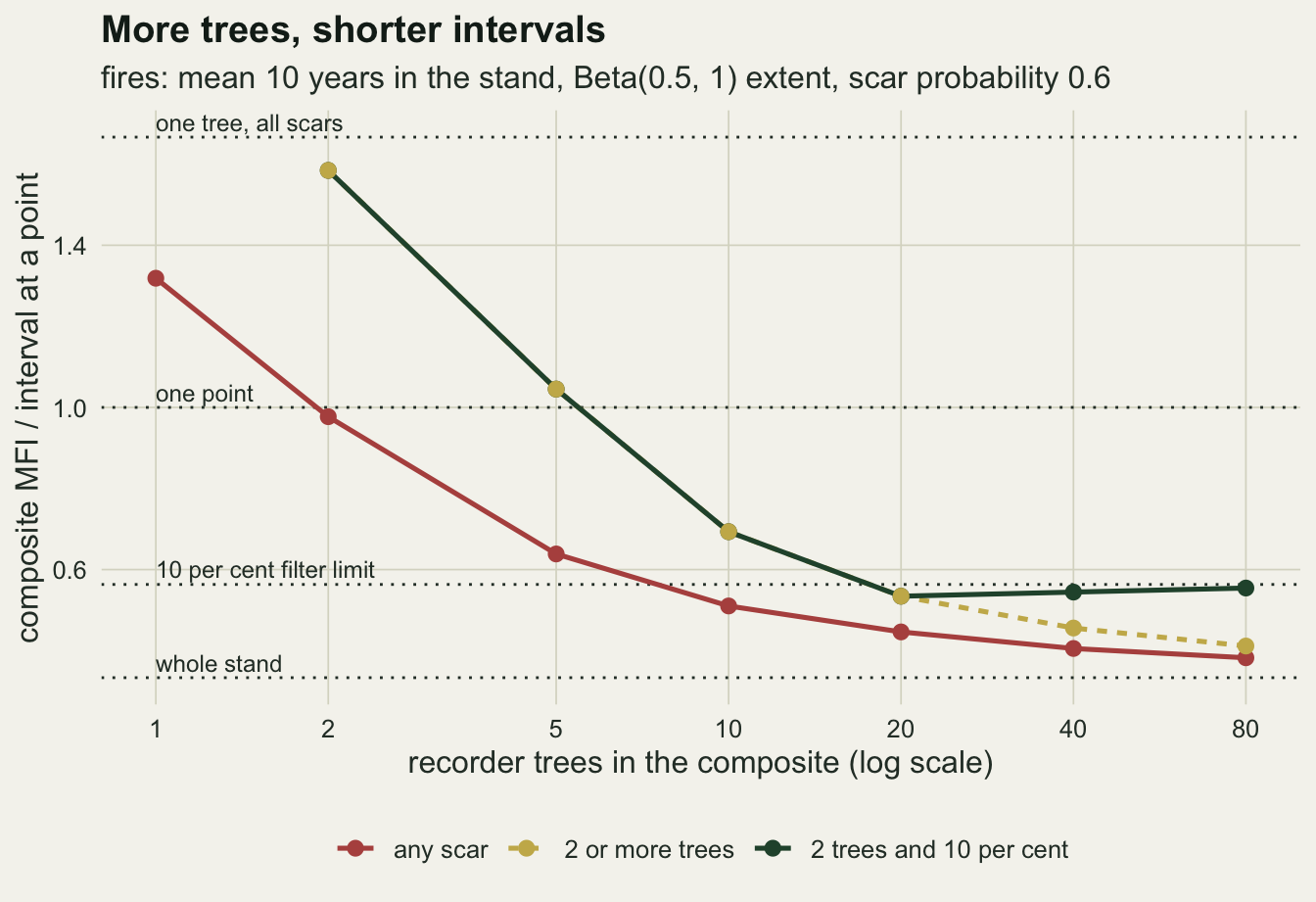
What to report
Say where the record starts. A record that starts at the first scar and one that starts at a date unrelated to fire support different estimators, and the difference is not a detail: censoring the gap before the first scar treats a length biased piece of an interval as an ordinary one, and at shape 1 it moved the median estimate to 1.075 of the true mean and the mean estimate to 1.405.
Give the number of fires and the record length next to the mean fire interval, not just the number of intervals. The ratio of the two is itself an estimate of the mean interval when the record window is unrelated to fire (a documentary start date, not necessarily the pith), it needs no distributional assumption, and in these simulations it had a root mean square error of 0.287 against 0.418 for the naive mean at shape 1 and four mean intervals. The advantage is not universal: at eight mean intervals and shape 1 the order reversed, 0.461 for the count against 0.415 for the naive mean, because the reciprocal of a Poisson count is skewed upward: the mean ratios there were 1.117 for the count and 0.965 for the naive mean. If the naive mean and the count estimate disagree strongly, the record is short relative to the fire interval, and the disagreement is the finding.
Report how many candidate records were excluded by a minimum fire rule. At two mean intervals the rule removed 0.673 of simulated records at shape 1, and every estimator computed from the survivors had a median of at most 0.730 of the true mean, because the survivors were chosen for having fires close together.
For a composite, report the number of recorder trees through time and the filter, and do not present a composite interval as the interval at a point. In the composite simulation the unfiltered estimate at 80 trees was 0.382 of the point interval and the ten per cent filtered estimate 0.554, and neither number depends only on how often a point burns.
Honest limits
The fire process is stationary. Real fire histories span land use changes, fire exclusion and climate shifts, and a record that ends in a century of suppression has a long final gap for reasons the renewal model does not know about. The count estimator and the censored fits both read a long final gap as evidence of long intervals; the naive mean, which ignores the final open gap, does not.
Scars are recorded without error. Real trees miss fires, record some fires only after a first wound has made them susceptible, and lose older scars to rot and later fires. The recorder status of a tree changes through time, which is why fire historians track recording years, and none of that is simulated.
The Weibull is the true interval distribution in every cell of the single-record simulation. The stationary likelihood was therefore fitted with the correct family, and at four and eight mean intervals its root mean square error still differed from the count estimator’s by at most 0.010; with a mixture of fire types or a hazard that does not follow a power law its position could only be expected to get worse, though that was not simulated. The count estimator’s own condition, a record window unrelated to the fire dates, is also assumed rather than tested: a sampler who chooses the most visibly scarred trees chooses records with many fires.
An inner-ring date is not automatically unrelated to fire. Trees often establish after a fire, and a fire in the first years of a tree’s life kills it rather than scarring it, so the span from pith to first scar is a fire-free period selected for being long. Treating it as a forward recurrence time, or counting from the pith in the length over fires estimator, then pushes the estimate up. The simulation opens every record at a random date and does not include this; it is the span Baker and Ehle argued should be included, and this selection is one reason that argument is disputed.
Trees in the composite are scarred independently given the fire extent. Real fires burn contiguous patches, so nearby trees share fates, and the number of trees needed before a filter levels off is likely to be larger for a clustered sample than for the scattered one simulated; that was not tested. The Beta(0.5, 1) fire size distribution and the scar probability of 0.6 are choices, and the level of the ten per cent filter follows from them by the closed form above.
The three fire rule and the ten per cent filter were applied as fixed rules. Published studies use a range of minimum sample depths, and some compute intervals only over the period when a set number of trees were recording; those rules change the numbers but not the direction of the selection effect.
References
Johnson EA, Gutsell SL 1994 Advances in Ecological Research 25:239-287 (10.1016/S0065-2504(08)60216-0)
Baker WL, Ehle D 2001 Canadian Journal of Forest Research 31(7):1205-1226 (10.1139/x01-046)
Grissino-Mayer HD 2000 International Journal of Wildland Fire 9(1):37-50 (10.1071/WF99004)