library(ggplot2)
library(patchwork)

te_paper  <- "#f5f4ee"
te_ink    <- "#16241d"
te_body   <- "#2c3a31"
te_forest <- "#275139"
te_rust   <- "#b5534e"
te_gold   <- "#c9b458"
te_line   <- "#dad9ca"

theme_datasheet <- function() {
  theme_minimal(base_size = 12) +
    theme(plot.background  = element_rect(fill = te_paper, colour = NA),
          panel.background = element_rect(fill = te_paper, colour = NA),
          panel.grid.major = element_line(colour = te_line, linewidth = 0.3),
          panel.grid.minor = element_blank(),
          text             = element_text(colour = te_body),
          plot.title       = element_text(colour = te_ink, face = "bold"),
          plot.subtitle    = element_text(colour = te_body),
          axis.text        = element_text(colour = te_body))
}Detection from a single drone flight
R
abundance
imperfect detection
N-mixture
survey design
simulation
ecology tutorial
One drone pass gives one count per tile, so abundance and detection separate only through the bend in a link function. Single-visit N-mixture limits in R.
A drone flies a survey block once. The mosaic is stitched, the thermal frames are counted, and every 50 metre tile ends up with one number: how many deer were visible in that tile on that morning. Some were under canopy and did not appear. The report needs total abundance, so somebody has to say what fraction was missed, and there is no second flight to say it with. That a pass misses animals is documented rather than assumed: Brack, Kindel and Oliveira went through the sources of bias in unmanned aerial survey counts in 2018.
The repeat-visit machinery on this site does not apply here. N-mixture models for abundance separates abundance from detection by visiting the same site several times and reading the spread between visits, and occupancy and detection covariates does the same for presence. The Royle-Nichols model makes the point sharply for the case with no covariates at all: with one visit the likelihood depends on abundance and detection only through their product, so the surface is an exact ridge and nothing can be estimated. Hierarchical distance sampling manages one visit, but it pays for it with a ruler: the distances inside each site carry the detection function. Those posts buy detection with repeat visits or with a ruler; a mosaic has neither, and what is left is the shape of a link function.
Solymos, Lele and Bayne showed in 2012 that a single visit is enough provided detection carries its own covariate, because the detection probability enters the mean count through a link that is not linear, and that curvature separates it from abundance. Knape and Korner-Nievergelt replied in 2015 that estimates from non-replicated surveys lean hard on exactly those assumptions, and Solymos and Lele answered in 2016 that the identifiability condition is mild and usually satisfied. All three are right about what they claim. This post is a demonstration of that method and of that argument, not a discovery: it runs the single-visit estimator on simulated one-pass surveys and measures how wide the answer is when the identification rests on curvature alone.
The measured piece is the width of the band on total abundance as a function of two things a survey planner controls or knows: how steeply detection responds to its covariate, and how many tiles the block holds. Canopy cover is the awkward case, because the same canopy that hides an animal from a thermal camera is also the canopy that holds the animals, so cover sits in both processes at once.
One flight per tile gives an ordinary Poisson count
The generating model is the standard N-mixture of Royle 2004 with one visit. Tile \(i\) holds \(N_i \sim \text{Poisson}(\lambda_i)\) animals and the mosaic shows \(y_i \sim \text{Binomial}(N_i, p_i)\) of them. Elevation \(x_1\) drives density and canopy cover \(x_2\) drives thermal detection:
\[\log \lambda_i = a + b\,x_{1i} \;(+\; b_2 x_{2i}), \qquad \text{logit}\, p_i = c + d\,x_{2i}.\]
The term in brackets is present only in what the post calls the shared arm, where cover drives density as well as detection. Thinning a Poisson count gives a Poisson count, so the marginal distribution of what the drone records is exactly
\[y_i \sim \text{Poisson}(\lambda_i p_i),\]
with no latent variable left to integrate out. The single-visit fit is therefore a Poisson likelihood in the four or five parameters, and it takes a fraction of a second.
a_true  <- log(2.5)
b_true  <- 0.6
c_true  <- 0.3
b2_true <- 0.5
d_grid  <- c(-0.4, -1.0, -1.8)
n_grid  <- c(200, 2000)
rep_small <- 400
rep_big   <- 150
rep_two   <- 150
rep_rho   <- 400
rho_grid  <- c(0, 0.5, 0.8, 0.95)
mc_se_small <- sqrt(0.25 / rep_small)
mc_se_big   <- sqrt(0.25 / rep_big)
set.seed(4001)
p_bar <- mean(plogis(c_true + d_grid[2] * rnorm(2e5)))set.seed(5501)
n_check <- 2e5
lam_chk <- 2.5
p_chk <- 0.4
n_lat <- rpois(n_check, lam_chk)
y_chk <- rbinom(n_check, n_lat, p_chk)
tab_obs <- tabulate(y_chk + 1L, nbins = 12) / n_check
tab_exp <- dpois(0:11, lam_chk * p_chk)
gap_marg <- max(abs(tab_obs - tab_exp))
se_marg <- max(sqrt(tab_exp * (1 - tab_exp) / n_check))
gap_in_se <- gap_marg / se_margThe identity is worth checking rather than repeating. Drawing 200000 tiles with a true mean of 2.5 animals and a detection probability of 0.4, the largest gap between the simulated frequency of a count and the Poisson probability with mean 1.0 is 0.00133, which is 1.2 times the largest Monte Carlo standard error among those twelve frequencies. The thinned counts are Poisson to simulation accuracy.
That identity is also the difficulty. The likelihood sees the data only through the mean function \(\lambda_i p_i\), so two parameter vectors that produce the same mean on every tile cannot be told apart. Write \(g(x_2) = \log \text{plogis}(c + d\,x_2)\), the contribution of detection to the log mean, and split it into its best linear approximation over the covariate distribution plus a remainder:
\[\log(\lambda_i p_i) = \underbrace{(a + g_0)}_{\text{intercept}} + b\,x_{1i} + \underbrace{(b_2 + g_1)}_{\text{slope on cover}} x_{2i} + \underbrace{r(x_{2i})}_{\text{curvature}}.\]
A linear model in the two covariates can read only three of those quantities. In the distinct-covariate arm there are four parameters to recover from three linear readings, and in the shared arm there are five. The deficit is closed by \(r(x_2)\), the part of the detection curve that no straight line reproduces. That remainder is the entire evidence for detection in a one-pass survey.
x_quad <- seq(-6, 6, length.out = 4001)
w_quad <- dnorm(x_quad) / sum(dnorm(x_quad))

decomp <- function(d_det) {
  g_fun <- log(plogis(c_true + d_det * x_quad))
  g0 <- sum(w_quad * g_fun)
  g1 <- sum(w_quad * g_fun * x_quad)
  r_fun <- g_fun - g0 - g1 * x_quad
  list(g = g_fun, g0 = g0, g1 = g1, r = r_fun,
       amp = sqrt(sum(w_quad * r_fun^2)))
}
dec_all  <- lapply(d_grid, decomp)
curv_amp <- vapply(dec_all, function(z) z$amp, 0)
lin_slope <- vapply(dec_all, function(z) z$g1, 0)

mu_bar   <- exp(a_true + b_true^2 / 2) * p_bar
coef_se  <- 1 / sqrt(n_grid * mu_bar)
lever    <- outer(curv_amp, coef_se, "/")
dimnames(lever) <- list(sprintf("%.1f", d_grid), sprintf("%d", n_grid))
With the detection intercept fixed at 0.3 and cover standard normal across tiles, the curvature amplitude is 0.0267 log units at a detection slope of -0.4, 0.1449 at -1.0, and 0.3715 at -1.8. Against that stands the precision of a log-mean coefficient, roughly one over the square root of the total expected count: 0.0545 on 200 tiles and 0.0172 on 2000, at an average recorded count of 1.68 animals per tile, which is what the distinct-covariate design gives at the middle detection slope.
The linear part of the same curve has slope -0.44 at a detection slope of -1.0, and in the shared arm that is precisely what the abundance coefficient on cover absorbs, leaving the curvature on its own.
The ratio of the two is the lever the estimator has to work with. On 200 tiles it is 0.49 at the shallow detection slope, 2.66 at the middle one and 6.82 at the steep one. A lever below one means the curvature that carries the whole identification is smaller than the noise on a coefficient, and no amount of care in the optimiser will retrieve it.
x_show <- seq(-3, 3, length.out = 241)
curve_df <- do.call(rbind, lapply(seq_along(d_grid), function(j) {
  g_fun <- log(plogis(c_true + d_grid[j] * x_show))
  data.frame(x2 = x_show, g = g_fun,
             lin = dec_all[[j]]$g0 + dec_all[[j]]$g1 * x_show,
             slope = factor(sprintf("%.1f", d_grid[j]),
                            levels = sprintf("%.1f", d_grid)))
}))
curve_df$resid <- curve_df$g - curve_df$lin
pal_d <- c(te_gold, te_forest, te_rust)

p_left <- ggplot(curve_df, aes(x2, g, colour = slope)) +
  geom_line(aes(y = lin), linetype = "dashed", linewidth = 0.5,
            show.legend = FALSE) +
  geom_line(linewidth = 0.9) +
  scale_colour_manual(values = pal_d, name = "detection slope",
                      guide = guide_legend(nrow = 1)) +
  labs(x = "canopy cover (standard deviations)",
       y = "log detection term",
       title = "The detection term",
       subtitle = "dashed: its best straight line") +
  theme_datasheet()

p_right <- ggplot(curve_df, aes(x2, resid, colour = slope)) +
  geom_hline(yintercept = 0, colour = te_line, linewidth = 0.4) +
  geom_line(linewidth = 0.9) +
  scale_colour_manual(values = pal_d, name = "detection slope",
                      guide = guide_legend(nrow = 1)) +
  labs(x = "canopy cover (standard deviations)",
       y = "curvature left over",
       title = "What the line misses",
       subtitle = "the whole evidence on detection") +
  theme_datasheet()

(p_left | p_right) + plot_layout(guides = "collect") +
  plot_annotation(theme = theme_datasheet() +
                    theme(legend.position = "bottom",
                          legend.direction = "horizontal"))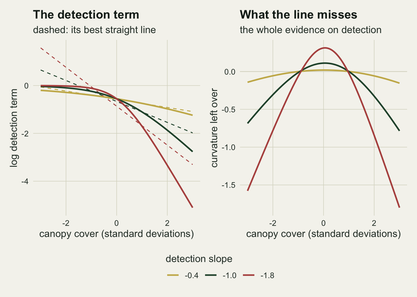
One flight with two distinct covariates
The estimator is a Poisson likelihood fitted by BFGS with an analytic gradient, and the standard errors come from the Hessian. Two details matter for honesty. Each data set is fitted from three starting values, differing in where the detection slope starts, and the best of the three is kept: nothing below is an optimiser that got stuck in the first place it landed. And a fit is counted as blown up when the estimated total exceeds fifty times the truth or the Hessian is singular, which is a failure the analyst would see on their own screen.
nll_sv <- function(th, y_obs, x1, x2, shared) {
  lin <- th[1] + th[2] * x1
  if (shared) lin <- lin + th[5] * x2
  mu <- exp(lin) * plogis(th[3] + th[4] * x2)
  if (any(!is.finite(mu)) || any(mu <= 0)) return(1e10)
  sum(mu) - sum(y_obs * log(mu))
}

gr_sv <- function(th, y_obs, x1, x2, shared) {
  lin <- th[1] + th[2] * x1
  if (shared) lin <- lin + th[5] * x2
  p_hat <- plogis(th[3] + th[4] * x2)
  mu <- exp(lin) * p_hat
  if (any(!is.finite(mu)) || any(mu <= 0)) return(rep(0, length(th)))
  resid_i <- y_obs - mu
  q_hat <- 1 - p_hat
  -c(sum(resid_i), sum(resid_i * x1), sum(resid_i * q_hat),
     sum(resid_i * q_hat * x2), sum(resid_i * x2))[seq_len(length(th))]
}

sim_tiles <- function(n_tile, shared, d_det, rho = 0) {
  x1 <- rnorm(n_tile)
  x2 <- rnorm(n_tile)
  if (rho != 0) x1 <- rho * x2 + sqrt(1 - rho^2) * x1
  lin <- a_true + b_true * x1
  if (shared) lin <- lin + b2_true * x2
  lam <- exp(lin)
  p_i <- plogis(c_true + d_det * x2)
  n_lat <- rpois(n_tile, lam)
  list(x1 = x1, x2 = x2, n_lat = n_lat,
       y1 = rbinom(n_tile, n_lat, p_i), y2 = rbinom(n_tile, n_lat, p_i))
}

fit_sv <- function(dat, shared) {
  gco <- glm.fit(cbind(1, dat$x1, dat$x2), dat$y1, family = poisson())$coefficients
  naive_cover <- unname(gco[3])
  starts <- list(c(gco[1] + log(2), gco[2], 0, 0, 0),
                 c(gco[1] + log(2), gco[2], 0,  naive_cover, 0),
                 c(gco[1] + log(2), gco[2], 0, -naive_cover, 0))
  best <- NULL
  for (st in starts) {
    fit <- try(optim(st[seq_len(4 + shared)], nll_sv, gr_sv, y_obs = dat$y1,
                     x1 = dat$x1, x2 = dat$x2, shared = shared, method = "BFGS",
                     hessian = TRUE, control = list(maxit = 500)), silent = TRUE)
    if (!inherits(fit, "try-error") && is.finite(fit$value) &&
        (is.null(best) || fit$value < best$value)) best <- fit
  }
  if (is.null(best)) return(c(NA, NA, NA, NA, naive_cover))
  th <- best$par
  lin <- th[1] + th[2] * dat$x1
  if (shared) lin <- lin + th[5] * dat$x2
  se_c <- tryCatch(suppressWarnings(sqrt(diag(solve(best$hessian)))[3]),
                   error = function(e) NA_real_)
  c(sum(exp(lin)) / sum(dat$n_lat), se_c, th[3], th[4], naive_cover)
}

cell_sv <- function(n_tile, shared, d_det, n_rep, seed, rho = 0) {
  set.seed(seed)
  out <- t(vapply(seq_len(n_rep),
                  function(i) fit_sv(sim_tiles(n_tile, shared, d_det, rho), shared),
                  numeric(5)))
  fin <- is.finite(out[, 1])
  usable <- fin & is.finite(out[, 2])
  data.frame(n_tile = n_tile, shared = shared, d_det = d_det, n_rep = n_rep,
             n_usable = sum(usable), rho = rho,
             med = median(out[fin, 1]),
             q10 = unname(quantile(out[fin, 1], 0.1)),
             q90 = unname(quantile(out[fin, 1], 0.9)),
             blow = mean(!usable | out[, 1] > 50),
             se_c = median(out[usable, 2]),
             wrong_sign = mean(out[usable, 4] > 0),
             naive = median(out[fin, 5]))
}
cells <- expand.grid(d_det = d_grid, shared = c(FALSE, TRUE), n_tile = n_grid)
sv_tab <- do.call(rbind, lapply(seq_len(nrow(cells)), function(i) {
n_rep <- if (cells$n_tile[i] == n_grid[1]) rep_small else rep_big
cell_sv(cells$n_tile[i], cells$shared[i], cells$d_det[i], n_rep, 24100 + i)
}))
sv_tab$width <- sv_tab$q90 / sv_tab$q10
pick <- function(n_tile, shared, d_det) {
sv_tab[sv_tab$n_tile == n_tile & sv_tab$shared == shared &
sv_tab$d_det == d_det, ]
}
dis_small <- pick(n_grid[1], FALSE, d_grid[2])
n_wrong_dis <- round(pick(n_grid[1], FALSE, d_grid[2])$n_usable *
pick(n_grid[1], FALSE, d_grid[2])$wrong_sign)
dis_big <- pick(n_grid[2], FALSE, d_grid[2])
sha_small <- pick(n_grid[1], TRUE, d_grid[2])
sha_big <- pick(n_grid[2], TRUE, d_grid[2])
flat_dis <- pick(n_grid[1], FALSE, d_grid[1])
steep_sha <- pick(n_grid[1], TRUE, d_grid[3])
steep_sha_big <- pick(n_grid[2], TRUE, d_grid[3])
steep_dis_big <- pick(n_grid[2], FALSE, d_grid[3])The replication was fixed before any of this ran: 400 surveys per cell at 200 tiles, 150 at 2000 and 150 in each two-flight cell below, so the Monte Carlo standard error of a reported share is at most 0.025 where a cell holds 400 surveys and 0.041 where it holds 150. No parameter was changed after seeing a result.
With elevation on density, cover on detection and nothing shared, the single-visit estimator works. Over 200 tiles at a detection slope of -1.0 the median ratio of estimated to true total abundance is 0.98, and the middle eight tenths of surveys fall between 0.81 and 1.59 times the truth. The fitted detection slope came out positive in 0 of the 400 surveys that returned a usable fit, and 0.2 per cent of fits blew up. On 2000 tiles the band tightens to 0.92 to 1.12 and the median standard error of the detection intercept falls from 0.66 to 0.20.
That is the Solymos, Lele and Bayne result reproduced: one count per site, no replication anywhere, and eight surveys in ten inside a band whose ends differ by a factor of 1.98. It is worth pausing on how strange that is against the Royle-Nichols ridge, where one visit gave nothing at all. The difference is the detection covariate, and specifically the bend it puts into the mean.
When canopy cover drives both processes
Now let cover raise density as well as lowering detection, with an abundance slope of 0.5 on the same standardised cover that carries a detection slope of -1.0. Nothing else changes. The model fitted is the correct one, including the cover term in the abundance part, so this is not misspecification: it is the same truth with one more parameter to find.
width_ratio_small <- sha_small$width / dis_small$width
width_ratio_big   <- sha_big$width / dis_big$width
se_ratio_small    <- sha_small$se_c / dis_small$se_c

wrong_n    <- c(sha_small$n_usable, sha_big$n_usable)
wrong_hit  <- round(wrong_n * c(sha_small$wrong_sign, sha_big$wrong_sign))
wrong_pool <- sum(wrong_hit) / sum(wrong_n)
wrong_se   <- sqrt(wrong_pool * (1 - wrong_pool) * sum(1 / wrong_n))
wrong_z    <- abs(sha_big$wrong_sign - sha_small$wrong_sign) / wrong_se

cost_big   <- c(sha_big$width / dis_big$width,
                steep_sha_big$width / steep_dis_big$width)
The estimator falls apart. Over 200 tiles the middle eight tenths of surveys now run from 0.48 to 55.6 times the true total, a band 58 times wider on the ratio scale than the distinct-covariate band at the same size and the same detection slope. 12.5 per cent of fits blew up, against 0.2 per cent before, and the median standard error of the detection intercept is 4.1 times larger. In 61 per cent of the surveys that returned a usable fit the detection slope came out positive: the model reports that thermal detection improves under canopy.
Raising the number of tiles helps and does not rescue it. At 2000 tiles, ten times the survey, the band is 0.79 to 3.52, still 3.7 times the width of the distinct-covariate band at the same size, and the fitted detection slope carries the wrong sign in 69 per cent of surveys, no better than at 200 tiles: the gap between the two shares is 1.6 standard errors of the difference, which settles nothing except that ten times the survey did not repair the sign. Identifiability is not the question: Solymos and Lele are right that the parameters are identified, since two different parameter vectors do give different mean functions. The question is how much of the likelihood surface lies within a hair of the maximum, and the answer is a long way.
A drone team has a reply to this, and it is a good one: the honest detection covariate is not canopy cover but the visible sky fraction over each tile, which the imagery itself measures, and that is a different variable from the cover that holds the deer. Where the two can be separated, the design is the distinct-covariate one above and it works. But sky fraction is close to one minus cover, so the two arms measured so far are the ends of a range and not the only two cases available. The middle of that range is a design in which the abundance covariate and the detection covariate are separate columns that happen to correlate, and the fitter above needs no change to run on it.
rho_tab <- do.call(rbind, lapply(seq_along(rho_grid), function(j)
  cell_sv(n_grid[1], FALSE, d_grid[2], rep_rho, 31100 + j, rho_grid[j])))
rho_tab$width <- rho_tab$q90 / rho_tab$q10
rho_last  <- nrow(rho_tab)
rho_cost  <- rho_tab$width[rho_last] / rho_tab$width[1]
rho_se_up <- rho_tab$se_c[rho_last] / rho_tab$se_c[1]
Over 200 tiles at a detection slope of -1.0, with 400 fresh surveys per cell, the middle eight tenths of estimates span a factor of 1.82 when the two covariates are uncorrelated, 2.23 at a correlation of 0.5, 3.01 at 0.8 and 5.49 at 0.95, while the median standard error of the detection intercept climbs from 0.67 to 1.28. The drone team’s reply survives the whole range: even at a correlation of 0.95 the band is a factor of 5.5, against 115 when one covariate carries both processes. It is not free either: the band widens 3.0 times and the detection standard error 1.9 times across that range, and at the top of it the band is no tighter than the factor of 4.46 the shared design reaches on 2000 tiles. The uncorrelated cell here is the distinct-covariate design of the previous section drawn again with its own seed, which is why its width is 1.82 and not 1.98. The next section is about what happens when the covariates can be separated but the detection response to the separated covariate is shallow.
nll_fixd <- function(th, d_fix, y_obs, x1, x2, shared) {
  lin <- th[1] + th[2] * x1
  if (shared) lin <- lin + th[4] * x2
  mu <- exp(lin) * plogis(th[3] + d_fix * x2)
  if (any(!is.finite(mu)) || any(mu <= 0)) return(1e10)
  sum(mu) - sum(y_obs * log(mu))
}

profile_d <- function(dat, shared, d_seq) {
  st0 <- c(log(2 * (mean(dat$y1) + 0.5)), 0, 0, 0)[seq_len(3 + shared)]
  walk <- function(idx, st) {
    out <- matrix(NA_real_, length(idx), 2)
    for (k in seq_along(idx)) {
      fit <- optim(st, nll_fixd, NULL, d_fix = d_seq[idx[k]], y_obs = dat$y1,
                   x1 = dat$x1, x2 = dat$x2, shared = shared,
                   method = "BFGS", control = list(maxit = 800))
      st <- fit$par
      lin <- fit$par[1] + fit$par[2] * dat$x1
      if (shared) lin <- lin + fit$par[4] * dat$x2
      out[k, ] <- c(fit$value, sum(exp(lin)) / sum(dat$n_lat))
    }
    out
  }
  mid <- which.min(abs(d_seq - d_grid[2]))
  up  <- walk(mid:length(d_seq), st0)
  dn  <- walk((mid - 1):1, st0)
  res <- rbind(dn[rev(seq_len(nrow(dn))), , drop = FALSE], up)
  data.frame(d_det = d_seq, devi = 2 * (res[, 1] - min(res[, 1])),
             ratio = res[, 2])
}

d_seq <- seq(-3, 3, length.out = 61)
set.seed(51515)
dat_dis <- sim_tiles(n_grid[1], FALSE, d_grid[2])
dat_sha <- sim_tiles(n_grid[1], TRUE,  d_grid[2])
prof_dis <- profile_d(dat_dis, FALSE, d_seq)
prof_sha <- profile_d(dat_sha, TRUE,  d_seq)
chi_cut <- qchisq(0.95, 1)
in_dis <- prof_dis[prof_dis$devi <= chi_cut, ]
in_sha <- prof_sha[prof_sha$devi <= chi_cut, ]
dis_nrange <- range(in_dis$ratio)
sha_nrange <- range(in_sha$ratio)
sha_devmax <- max(prof_sha$devi)
dis_devmax <- max(prof_dis$devi)
A profile makes the shape visible on a single survey. Fixing the detection slope at each value of a grid and maximising over everything else gives the profile deviance, and twice the drop from the maximum is on the chi-squared scale with one degree of freedom, so 3.84 is the usual 95 per cent cut. On the distinct-covariate survey the profile has a clear minimum, rises to 178 across the grid, and the slopes inside the cut imply totals between 0.79 and 1.37 times the truth. On the shared-covariate survey the deviance never exceeds 1.2 anywhere on the grid, so every detection slope from -3 to +3 is inside the interval, both signs included, and the implied totals inside the cut run from 0.47 to 53565 times the truth. The interval on abundance is open at the top: the data do not close it.
prof_all <- rbind(cbind(prof_dis, arm = "distinct covariates"),
                  cbind(prof_sha, arm = "cover on both"))
prof_all$arm <- factor(prof_all$arm,
                       levels = c("distinct covariates", "cover on both"))
pal_arm <- c("distinct covariates" = te_forest, "cover on both" = te_rust)

p_d <- ggplot(prof_all, aes(d_det, devi, colour = arm)) +
  geom_hline(yintercept = chi_cut, linetype = "dashed",
             colour = te_body, linewidth = 0.5) +
  geom_line(linewidth = 0.9) +
  scale_colour_manual(values = pal_arm, name = NULL,
                      guide = guide_legend(nrow = 1)) +
  coord_cartesian(ylim = c(0, 20)) +
  labs(x = "detection slope held fixed", y = "profile deviance",
       title = "One survey, profiled",
       subtitle = "dashed: the 95 per cent cut") +
  theme_datasheet()

p_n <- ggplot(prof_all[prof_all$devi <= 8, ], aes(ratio, devi, colour = arm)) +
  geom_hline(yintercept = chi_cut, linetype = "dashed",
             colour = te_body, linewidth = 0.5) +
  geom_line(linewidth = 0.9) +
  scale_colour_manual(values = pal_arm, name = NULL,
                      guide = guide_legend(nrow = 1)) +
  scale_x_log10() +
  labs(x = "estimated total / true total", y = "profile deviance",
       title = "The cost in abundance",
       subtitle = "the shared arm stays flat") +
  theme_datasheet()

(p_d | p_n) + plot_layout(guides = "collect") +
  plot_annotation(theme = theme_datasheet() +
                    theme(legend.position = "bottom",
                          legend.direction = "horizontal"))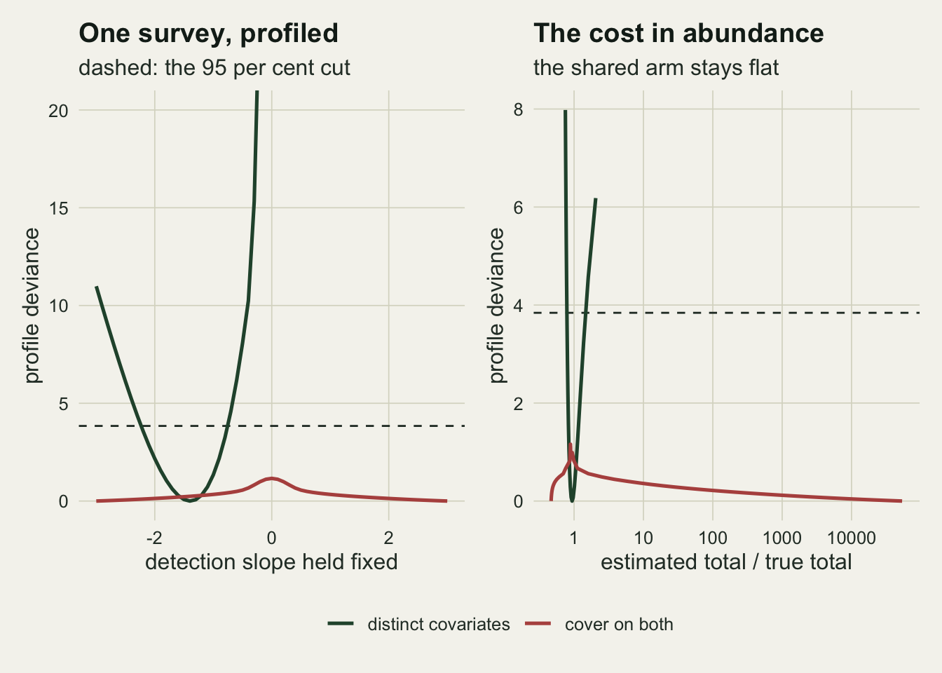
The lever is the curvature, not the covariate list
It would be comfortable to conclude that distinct covariates are the requirement. They are not. Holding the covariates distinct and flattening the detection response to a slope of -0.4 breaks the estimator on its own: the band over 200 tiles runs from 0.64 to 60 times the truth, 47 times wider than at a slope of -1.0, with 12 per cent of fits blown up. The curvature amplitude at that slope was 0.027 against a coefficient precision of 0.055: there was nothing to read.
The same argument runs the other way. Steepening the slope to -1.8 while keeping cover in both processes pulls the shared arm partway back, to 0.58 to 18.5 over 200 tiles. It is still far worse than any distinct-covariate cell, because the shared arm has to fund one extra parameter out of the same curvature, but at a block of this size the detection slope, not the covariate list, is what the design turns on.
At 2000 tiles that stops being true. The shared band spans a factor of 4.46 at a detection slope of -1.0 and 4.78 at -1.8, so steepening the response buys nothing there, while the covariate list still costs a factor of 3.7 and 4.4 on the band at those two slopes. Once the block is large enough for the curvature to be read at all, what is left is the extra parameter, and no detection slope takes it away.
band_df <- sv_tab
band_df$arm <- factor(ifelse(band_df$shared, "cover on both",
                             "distinct covariates"),
                      levels = c("distinct covariates", "cover on both"))
band_df$steep <- abs(band_df$d_det)
band_df$panel <- factor(sprintf("%d tiles", band_df$n_tile),
                        levels = sprintf("%d tiles", n_grid))

ggplot(band_df, aes(steep, med, colour = arm)) +
  geom_hline(yintercept = 1, linetype = "dashed",
             colour = te_body, linewidth = 0.5) +
  geom_errorbar(aes(ymin = q10, ymax = q90), width = 0.2,
                linewidth = 0.7, position = position_dodge(width = 0.3)) +
  geom_point(size = 2.4, position = position_dodge(width = 0.3)) +
  facet_wrap(~panel) +
  scale_colour_manual(values = pal_arm, name = NULL) +
  scale_y_log10() +
  scale_x_continuous(breaks = abs(d_grid)) +
  labs(x = "steepness of the detection slope",
       y = "estimated total / true total",
       title = "What one flight can promise",
       subtitle = "points: median; bars: middle eight tenths of surveys") +
  theme_datasheet() +
  theme(legend.position = "bottom",
        strip.text = element_text(colour = te_ink, face = "bold"))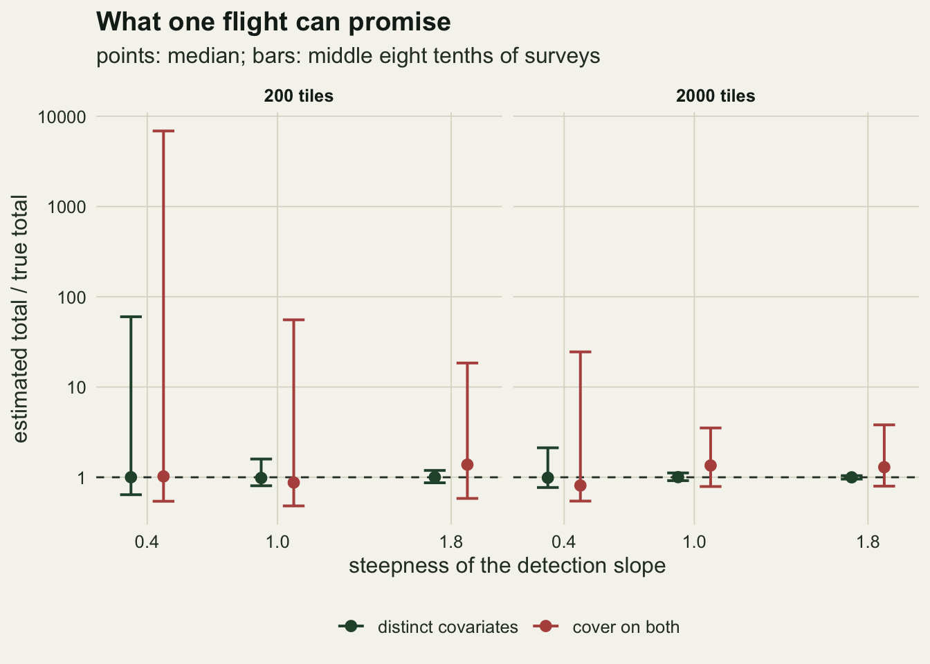
What a second flight buys
The remedy is the one the repeat-visit posts already use, and the point of measuring it here is the size of the gain rather than its existence. Flying the same block twice on the same morning turns each tile into two counts of the same \(N_i\), the latent abundance has to be marginalised out again, and the model is the ordinary two-visit N-mixture.
n_max <- 60L
grid_n <- 0:n_max
sd_log <- sqrt(b_true^2 + b2_true^2)
p_over <- sum(w_quad * ppois(n_max, exp(a_true + sd_log * x_quad),
                             lower.tail = FALSE))

pre_k2 <- function(dat) {
  n_tile <- length(dat$y1)
  n_mat <- matrix(grid_n, n_tile, n_max + 1L, byrow = TRUE)
  list(n_mat = n_mat, ysum = dat$y1 + dat$y2,
       const = lchoose(n_mat, dat$y1) + lchoose(n_mat, dat$y2) -
         lgamma(n_mat + 1))
}

nll_k2 <- function(th, pre, x1, x2, shared) {
  lin <- th[1] + th[2] * x1
  if (shared) lin <- lin + th[5] * x2
  lam <- exp(lin)
  p_hat <- plogis(th[3] + th[4] * x2)
  if (any(!is.finite(lam)) || any(lam <= 0) || any(lam > 1e6)) return(1e10)
  lq <- log1p(-p_hat)
  tot <- pre$const + pre$n_mat * (log(lam) + 2 * lq) +
    (-lam + pre$ysum * (log(p_hat) - lq))
  top <- tot[cbind(seq_along(lam), max.col(tot, "first"))]
  ll <- top + log(rowSums(exp(tot - top)))
  if (any(!is.finite(ll))) return(1e10)
  -sum(ll)
}

fit_k2 <- function(dat, shared) {
  pre <- pre_k2(dat)
  st <- c(log(2 * (mean(dat$y1) + 0.5)), 0, 0, 0, 0)[seq_len(4 + shared)]
  fit <- try(optim(st, nll_k2, NULL, pre = pre, x1 = dat$x1, x2 = dat$x2,
                   shared = shared, method = "BFGS", hessian = TRUE,
                   control = list(maxit = 500)), silent = TRUE)
  if (inherits(fit, "try-error")) return(c(NA, NA, NA, NA))
  th <- fit$par
  lin <- th[1] + th[2] * dat$x1
  if (shared) lin <- lin + th[5] * dat$x2
  se_c <- tryCatch(suppressWarnings(sqrt(diag(solve(fit$hessian)))[3]),
                   error = function(e) NA_real_)
  c(sum(exp(lin)) / sum(dat$n_lat), se_c, th[3], th[4])
}

cell_k2 <- function(shared, seed) {
  set.seed(seed)
  out <- t(vapply(seq_len(rep_two),
                  function(i) fit_k2(sim_tiles(n_grid[1], shared, d_grid[2]),
                                     shared),
                  numeric(4)))
  fin <- is.finite(out[, 1])
  usable <- fin & is.finite(out[, 2])
  data.frame(shared = shared, med = median(out[fin, 1]),
             q10 = unname(quantile(out[fin, 1], 0.1)),
             q90 = unname(quantile(out[fin, 1], 0.9)),
             blow = mean(!usable | out[, 1] > 50),
             se_c = median(out[usable, 2]),
             wrong_sign = mean(out[usable, 4] > 0),
             n_usable = sum(usable))
}
k2_tab <- rbind(cell_k2(FALSE, 26001), cell_k2(TRUE, 26002))
k2_dis <- k2_tab[!k2_tab$shared, ]
k2_sha <- k2_tab[k2_tab$shared, ]
se_gain_sha <- sha_small$se_c / k2_sha$se_c
se_gain_dis <- dis_small$se_c / k2_dis$se_c
n_wrong_k2 <- round(k2_sha$n_usable * k2_sha$wrong_sign)
The marginalisation runs on a grid of abundances up to 60, which the latent abundance of a tile exceeds in about one tile in 35 thousand in the shared arm, and it is vectorised over tiles, so the whole arm costs a few seconds.
Two flights over the shared-covariate block cut the median standard error of the detection intercept from 2.69 to 0.20, a factor of 13, and pull the abundance band from 0.48 to 55.6 back to 0.85 to 1.22. On one flight the fitted detection slope came out positive in 61 per cent of usable fits; on two, in 0 of the 150 usable fits. On the distinct-covariate block, where one flight already worked, the second flight still cuts the detection standard error by a factor of 4.3 and narrows the band to 0.93 to 1.07.
The two routes to a narrower band do not compare on any simple cost scale, because the second flight over a 200 tile block costs one more sortie while the ten-fold block costs a different survey altogether. But the direction is worth stating plainly: on the shared-covariate design, ten times as many tiles bought a band of 0.79 to 3.52 while one repeat flight over the original block bought 0.85 to 1.22.
flight_df <- rbind(
  data.frame(flights = 1, arm = c("distinct covariates", "cover on both"),
             se_c = c(dis_small$se_c, sha_small$se_c),
             med = c(dis_small$med, sha_small$med),
             q10 = c(dis_small$q10, sha_small$q10),
             q90 = c(dis_small$q90, sha_small$q90)),
  data.frame(flights = 2, arm = c("distinct covariates", "cover on both"),
             se_c = c(k2_dis$se_c, k2_sha$se_c),
             med = c(k2_dis$med, k2_sha$med),
             q10 = c(k2_dis$q10, k2_sha$q10),
             q90 = c(k2_dis$q90, k2_sha$q90)))
flight_df$arm <- factor(flight_df$arm,
                        levels = c("distinct covariates", "cover on both"))

p_se <- ggplot(flight_df, aes(flights, se_c, colour = arm)) +
  geom_line(linewidth = 0.9) +
  geom_point(size = 2.6) +
  scale_colour_manual(values = pal_arm, name = NULL,
                      guide = guide_legend(nrow = 1)) +
  scale_x_continuous(breaks = c(1, 2)) +
  scale_y_log10() +
  labs(x = "flights over the block", y = "median SE of detection intercept",
       title = "What the repeat buys",
       subtitle = "two hundred tiles") +
  theme_datasheet()

p_band <- ggplot(flight_df, aes(flights, med, colour = arm)) +
  geom_hline(yintercept = 1, linetype = "dashed",
             colour = te_body, linewidth = 0.5) +
  geom_errorbar(aes(ymin = q10, ymax = q90), width = 0.12, linewidth = 0.7,
                position = position_dodge(width = 0.18)) +
  geom_point(size = 2.4, position = position_dodge(width = 0.18)) +
  scale_colour_manual(values = pal_arm, guide = "none") +
  scale_x_continuous(breaks = c(1, 2)) +
  scale_y_log10() +
  labs(x = "flights over the block", y = "estimated total / true total",
       title = "And to abundance",
       subtitle = "bars: middle eight tenths") +
  theme_datasheet()

(p_se | p_band) + plot_layout(guides = "collect") +
  plot_annotation(theme = theme_datasheet() +
                    theme(legend.position = "bottom",
                          legend.direction = "horizontal"))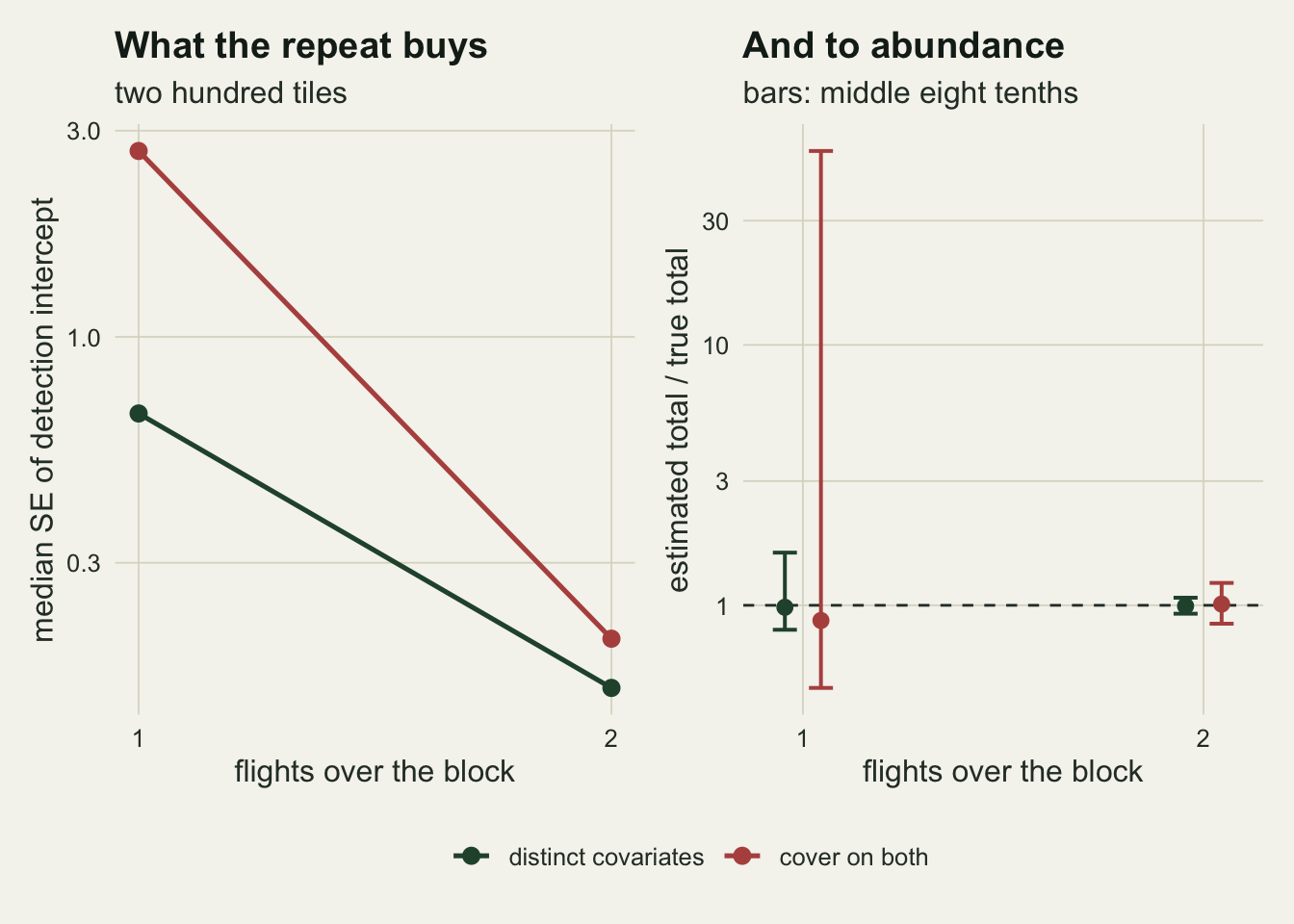
What a habitat model of the raw counts reports
A team that does not fit a detection model at all will regress the tile counts on the two covariates with a Poisson generalised linear model and call the coefficients habitat effects. That model is misspecified, because the log mean is not linear in cover, but it converges and prints a table.
naive_dis <- dis_small$naive
naive_sha <- sha_small$naive
naive_shift <- naive_sha - naive_dis
On the distinct-covariate surveys the naive cover coefficient is -0.37 in the median, although the true abundance slope on cover is zero: the whole coefficient is detection in disguise. On the shared-covariate surveys, where the true abundance slope on cover is +0.5, the naive coefficient is +0.05. A density effect of +0.5 and a detection effect of the opposite sign have very nearly cancelled, and the printed table says cover does not matter. The difference between the two arms is +0.42, which recovers most of the abundance slope but not all of it, because the nonlinear detection term does not split cleanly into a linear piece.
What to report
Compute the lever before the flight, not after. The curvature amplitude of the detection term at the slope and intercept you expect, divided by one over the square root of the total count you expect to record, is three numbers of arithmetic and it tells you whether the design has anything to estimate detection with. At a lever of 0.49 the estimator gave a band of 0.64 to 60 times the truth; at 6.82 it gave 0.87 to 1.19.
Say which covariates enter which process, and mean it. The difference between the two arms of this post is one slope, 0.5 on cover in the abundance model, and it moved the abundance band from a factor of 1.98 to a factor of 115. A single-visit estimate is only as good as the claim that the detection covariate is not also a density covariate, and that claim is ecological, not statistical.
Report the profile interval for total abundance, not the Wald one. The shared-covariate profile in this post never rose above 1.2 deviance units anywhere on the slope grid, so the honest interval had no upper end, while a Hessian-based standard error would have printed a finite number.
Give the sign of the fitted detection slope a hard look. In the shared arm it disagreed with the truth in 61 per cent of usable fits at 200 tiles and 69 per cent at 2000. A detection model that says animals are easier to see under canopy is not a result, it is the ridge talking, and fitting from several starting values does not fix it because the second mode is a genuine competitor on the likelihood.
Fly the block twice if the block is small and the covariates overlap. Two flights over 200 tiles gave a tighter answer, 0.85 to 1.22, than one flight over 2000 tiles did, 0.79 to 3.52.
Honest limits
The detection covariate here is standard normal and continuous, which is the case Solymos and Lele’s identifiability condition is stated for. A covariate recorded in three cover classes gives the curve only three points to bend through, and the lever computed above is then an overstatement of what the data hold. Nothing in this post measures the discrete case.
The abundance distribution is Poisson and the fitted model knows it. Real tile counts are overdispersed, and a negative binomial abundance adds a dispersion parameter that has to come out of the same curvature; N-mixture reliability and the detection trade-off shows that this parameter is barely identified even with repeat visits. The single-visit bands here should be read as the best case in that respect.
The link is logit in both truth and fit. Knape and Korner-Nievergelt’s central point is that a single-visit estimate depends on the link being the right shape, because the shape is the evidence. A cloglog truth fitted with a logit, or a detection response that is quadratic in cover, changes the curvature itself, and this post holds the link fixed and varies only its steepness. That is a deliberate restriction and it makes the results here optimistic.
The two flights are the same morning with no movement between them, so closure holds exactly and the only new information is a second binomial draw. Animals that move between flights break the two-visit N-mixture in the usual way, and the gain reported above is an upper bound on what a real repeat delivers.
The correlated arm varies the correlation between the two covariates at one block size and one detection slope, with both covariates jointly normal. A sky fraction and a cover fraction are bounded and are related to each other by something closer to a curve than a correlation, so that arm maps the direction of the cost rather than its size on a real block.
Tiles are independent, and each tile draws its covariates without reference to its neighbours. Real cover is spatially autocorrelated and so is deer density, which reduces the effective number of tiles without reducing the nominal one. Every band in this post would be wider on a real block of the same size, and how much wider depends on the correlation range against the tile size.
The blow-up rule is a threshold at fifty times the truth, chosen before the runs. It is a summary of a failure that has no natural scale: in the worst cell the estimated total exceeded the truth by orders of magnitude, and a different threshold would move the reported share without changing anything about the picture. The band, which was computed over all fits that returned a finite estimate, carries the same information without the threshold.
Total abundance is summed over the same tiles the survey covered, so nothing here concerns extrapolation to unflown ground. The ratio reported throughout is the estimated sum of fitted densities over the true realised total, which is the quantity a block-level report actually contains.
References
Royle JA 2004 Biometrics 60(1):108-115 (10.1111/j.0006-341X.2004.00142.x)
Solymos P, Lele S, Bayne E 2012 Environmetrics 23(2):197-205 (10.1002/env.1149)
Knape J, Korner-Nievergelt F 2015 Methods in Ecology and Evolution 6(3):298-306 (10.1111/2041-210X.12329)
Solymos P, Lele SR 2016 Methods in Ecology and Evolution 7(2):196-205 (10.1111/2041-210X.12432)
Brack IV, Kindel A, Oliveira LFB 2018 Methods in Ecology and Evolution 9(8):1864-1873 (10.1111/2041-210X.13026)