Constrained ordination with distance-based RDA in R

Where NMDS shows all the compositional variation and lets you overlay environment afterward, distance-based RDA builds the ordination from your predictors and tests what they explain.

The ordination and hypothesis-testing posts shared a shape: build an unconstrained map of composition, then bring the environment to it, either as envfit() arrows or as an adonis2() test. Constrained ordination turns that around. Instead of arranging sites by whatever varies most and checking the environment afterward, it builds the axes out of the predictors themselves, so the picture shows only the variation those predictors can account for. Distance-based RDA, dbrda(), is the version that works from a dissimilarity such as Bray-Curtis, which makes it the natural constrained partner to everything in the previous two posts.

A dataset with two gradients

The data is synthetic so the structure is known. Forty sites carry two measured variables, soil moisture and soil nitrogen, drawn independently of each other. Fourteen species each respond to both, peaking at their own point along moisture and at a separate point along nitrogen. Because the two gradients are independent by construction, a good method should pull them apart and credit each with its own share of the pattern.

library(vegan)
library(ggplot2)
library(dplyr)

set.seed(20)
n <- 40
moisture <- round(runif(n, 0, 10), 1)
nitrogen <- round(runif(n, 0, 10), 1)

species <- sprintf("sp%02d", 1:14)
opt_m <- seq(1, 9, length.out = 14)            # moisture optimum per species
opt_n <- sample(seq(1, 9, length.out = 14))    # nitrogen optimum, independent of moisture
w <- 2.3
lambda <- sapply(seq_along(species), function(i)
  12 * exp(-((moisture - opt_m[i])^2 + (nitrogen - opt_n[i])^2) / (2 * w^2)))
comm <- matrix(rpois(length(lambda), as.vector(lambda)), nrow = n)
colnames(comm) <- species
rownames(comm) <- sprintf("S%02d", 1:n)

env <- data.frame(moisture = moisture, nitrogen = nitrogen)
comm[1:5, 1:7]

    sp01 sp02 sp03 sp04 sp05 sp06 sp07
S01    0    0    1    0    0    0    1
S02    0    0    0    3    0    0    0
S03    7    1   12    6    7    8    3
S04    0    1   11    0    5    7    2
S05    0    0    0    0    2    1    2

Building the model

dbrda() takes a formula with the community on the left and the predictors on the right, plus the dissimilarity to use. It computes the Bray-Curtis distances, then finds the axes through that distance space that the predictors can explain, leaving the rest as unconstrained residual structure.

mod <- dbrda(comm ~ moisture + nitrogen, data = env, distance = "bray")
mod

Call: dbrda(formula = comm ~ moisture + nitrogen, data = env, distance =
"bray")

              Inertia Proportion Rank RealDims
Total          9.8765     1.0000              
Constrained    5.5768     0.5647    2        2
Unconstrained  4.2997     0.4353   37       21

Inertia is squared Bray distance

Eigenvalues for constrained axes:
dbRDA1 dbRDA2 
3.1394 2.4374 

Eigenvalues for unconstrained axes:
  MDS1   MDS2   MDS3   MDS4   MDS5   MDS6   MDS7   MDS8 
1.6793 0.5864 0.5176 0.4716 0.2922 0.2687 0.2427 0.2012 
(Showing 8 of 37 unconstrained eigenvalues)

The summary splits the total inertia into a constrained part and an unconstrained part. The constrained rows are the variation that moisture and nitrogen jointly account for; the unconstrained rows are what is left. Here the two predictors carry a little over half of the total, and the constrained side has exactly two axes, one per predictor, named dbRDA1 and dbRDA2.

How much is explained

The constrained proportion is the headline number, but raw proportions climb whenever you add predictors, whether or not they matter. RsquareAdj() corrects for that, the same way adjusted R-squared does in a linear model, and the adjusted figure is the one to quote.

RsquareAdj(mod)

$r.squared
[1] 0.564657

$adj.r.squared
[1] 0.5411249

About 56 percent of the compositional variation is constrained, and the adjusted value stays close to it (near 0.54), because two predictors against forty sites is not a demanding ratio.

Is the model significant?

The proportion tells you the size of the effect; permutation tests tell you whether it beats chance. anova() on a dbrda object reshuffles the data many times and compares. Run it three ways: the whole model, then each term, then each axis.

set.seed(20)
anova(mod, permutations = 999)

Permutation test for dbrda under reduced model
Permutation: free
Number of permutations: 999

Model: dbrda(formula = comm ~ moisture + nitrogen, data = env, distance = "bray")
         Df SumOfSqs      F Pr(>F)    
Model     2   5.5768 23.995  0.001 ***
Residual 37   4.2997                  
---
Signif. codes:  0 '***' 0.001 '**' 0.01 '*' 0.05 '.' 0.1 ' ' 1

set.seed(20)
anova(mod, by = "terms", permutations = 999)

Permutation test for dbrda under reduced model
Terms added sequentially (first to last)
Permutation: free
Number of permutations: 999

Model: dbrda(formula = comm ~ moisture + nitrogen, data = env, distance = "bray")
         Df SumOfSqs      F Pr(>F)    
moisture  1   3.1164 26.818  0.001 ***
nitrogen  1   2.4604 21.172  0.001 ***
Residual 37   4.2997                  
---
Signif. codes:  0 '***' 0.001 '**' 0.01 '*' 0.05 '.' 0.1 ' ' 1

set.seed(20)
anova(mod, by = "axis", permutations = 999)

Permutation test for dbrda under reduced model
Forward tests for axes
Permutation: free
Number of permutations: 999

Model: dbrda(formula = comm ~ moisture + nitrogen, data = env, distance = "bray")
         Df SumOfSqs      F Pr(>F)    
dbRDA1    1   3.1394 27.015  0.001 ***
dbRDA2    1   2.4374 21.542  0.001 ***
Residual 37   4.2997                  
---
Signif. codes:  0 '***' 0.001 '**' 0.01 '*' 0.05 '.' 0.1 ' ' 1

The whole model is significant (pseudo-F around 24, p = 0.001). Split by term, moisture and nitrogen are each highly significant on their own, with similar F values, which fits the way they were built as two real and independent drivers. Split by axis, both constrained axes carry signal worth keeping, so a two-dimensional plot is justified rather than just convenient.

The biplot

A constrained ordination is read as a biplot: site points placed on the constrained axes, and the predictors drawn as arrows pointing in the direction each one increases. Colouring the points by moisture and sizing them by nitrogen lets you check the arrows against the raw values.

scl <- 2
site_sc <- as.data.frame(scores(mod, display = "sites", scaling = scl, choices = 1:2))
bp      <- as.data.frame(scores(mod, display = "bp",    scaling = scl, choices = 1:2))
names(site_sc) <- c("AX1", "AX2")
names(bp)      <- c("AX1", "AX2")
site_sc$moisture <- moisture
site_sc$nitrogen <- nitrogen

# scale the predictor arrows to sit over the site cloud
mul <- 0.9 * max(abs(as.matrix(site_sc[, 1:2]))) / max(sqrt(rowSums(bp^2)))
bp$lab <- rownames(bp)
bp$x <- bp$AX1 * mul
bp$y <- bp$AX2 * mul

eig <- mod$CCA$eig
lab1 <- sprintf("dbRDA1 (%.0f%% of fitted)", 100 * eig[1] / sum(eig))
lab2 <- sprintf("dbRDA2 (%.0f%% of fitted)", 100 * eig[2] / sum(eig))

ggplot(site_sc, aes(AX1, AX2)) +
  geom_hline(yintercept = 0, color = "#e2e1d4") +
  geom_vline(xintercept = 0, color = "#e2e1d4") +
  geom_point(aes(color = moisture, size = nitrogen)) +
  geom_segment(data = bp, aes(x = 0, y = 0, xend = x, yend = y), inherit.aes = FALSE,
               arrow = arrow(length = unit(0.2, "cm")), color = "#16241d", linewidth = 0.9) +
  geom_text(data = bp, aes(x = x, y = y, label = lab), inherit.aes = FALSE,
            color = "#16241d", fontface = "bold", vjust = -0.6, size = 3.6) +
  scale_color_gradient(low = "#c9b458", high = "#1d5b4e", name = "Moisture") +
  scale_size_continuous(range = c(1.3, 5), name = "Nitrogen") +
  labs(x = lab1, y = lab2) +
  coord_equal() +
  theme_minimal(base_size = 12)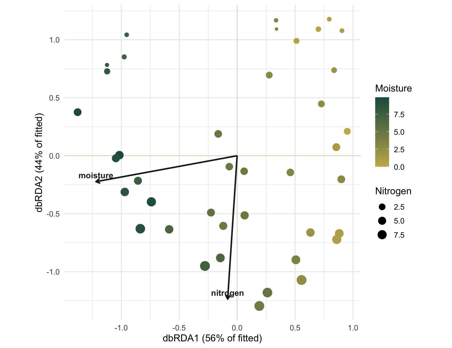

Figure 1: Distance-based RDA biplot. Sites are coloured by moisture and sized by nitrogen; arrows show the two predictors. The first axis tracks moisture, the second nitrogen, and the arrows sit at almost a right angle because the gradients are independent.

The first axis lines up with moisture: dry gold sites on one side, wet green ones on the other. The second axis lines up with nitrogen, and the point sizes grow along it. The two arrows meet at close to a right angle, the visual signature of predictors that vary independently. If moisture and nitrogen had been correlated in the field, the arrows would have drawn together, and the constrained axes would have struggled to separate their effects.

How this differs from NMDS and PERMANOVA

The three approaches answer different questions about the same kind of data. NMDS is unconstrained: it shows the full compositional structure and asks nothing of the environment until you overlay it with envfit(), which makes it the tool for exploring what is there. PERMANOVA tests whether named predictors explain composition but returns no map. Distance-based RDA does both at once: the anova() output is the test, and the biplot is the picture, but the picture shows only the slice of variation the predictors govern, not everything in the data. Reach for NMDS when you want to see all the structure and form hypotheses, and for dbrda() when you already have the predictors and want to model, measure, and display their effect directly.

Where to go next

capscale() is the close sibling of dbrda(), also distance-based, differing mainly in how each treats the negative eigenvalues that non-Euclidean distances can produce. A Condition() term partials out covariates you want to control for rather than test, and varpart() splits the explained variation among several predictor sets to show how much each contributes alone and how much they share. All of them build on the same move made here: let the predictors define the ordination, then test what they are worth.