Choosing priors: flat is not uninformative

Why vague priors can be strongly informative, in base R: flat logit priors on occupancy probability and the variance-prior trap in a hierarchical model.

The wish behind a vague prior is honest: let the data speak, do not smuggle in an answer. The mistake is thinking that a wide, flat distribution says nothing. A prior is a statement about a parameter on a particular scale, and flatness does not survive a change of scale. A prior that looks agnostic where you wrote it can be an opinionated prior everywhere you actually look. This post shows two versions of that failure in base R, both from scratch: a flat prior on a logit that turns into a strong prior on a probability, and the family of “vague” variance priors that never settle on a single noninformative answer.

A flat prior on the logit is a strong prior on the probability

Occupancy and detection probabilities are modelled on the logit scale, where a coefficient can run over the whole real line. The reflex is to put a wide normal prior there, say theta ~ N(0, sigma) with a large sigma, and call it vague. But the quantity we care about is the probability p = plogis(theta), and the implied density of p follows by change of variables.

# implied prior density of p = plogis(theta) when theta ~ N(0, s)
implied_p <- function(p, s) dnorm(qlogis(p), 0, s) / (p * (1 - p))

sig       <- c(1.5, 2.5, 10)
tail_mass <- sapply(sig, function(s) 2 * pnorm(qlogis(0.05), 0, s))  # P(p<.05 or p>.95)
names(tail_mass) <- paste0("N(0,", sig, ")")
round(tail_mass, 3)

N(0,1.5) N(0,2.5)  N(0,10) 
   0.050    0.239    0.768 

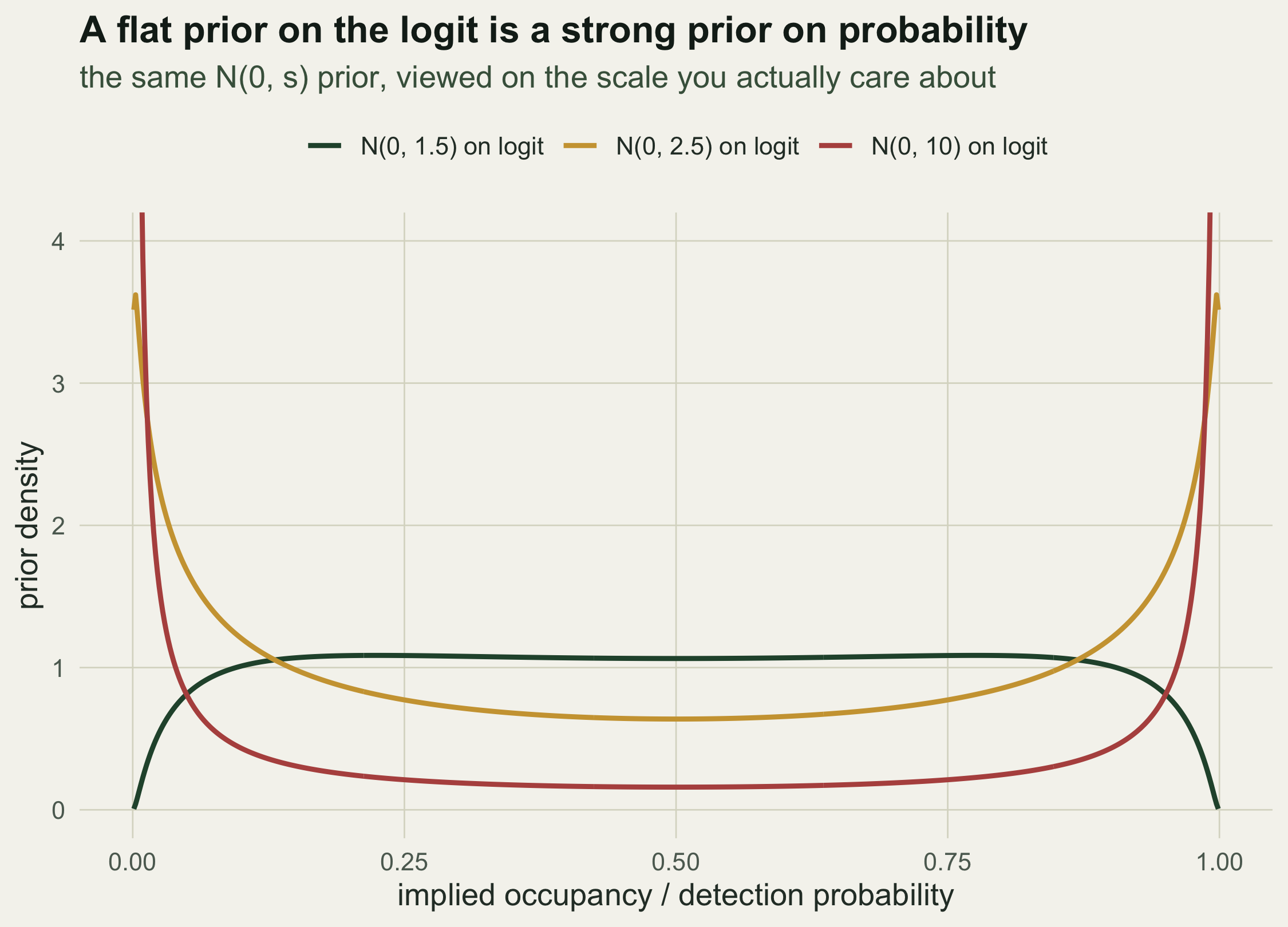
A wider prior does not spread the probability out evenly; it pushes it into the corners. Under N(0, 10), taken as vague on the logit, 77% of the prior probability sits below 0.05 or above 0.95: the prior believes, before seeing any data, that the species is almost certainly absent or almost certainly present. The gentler N(0, 1.5) leaves only 5% in those tails and is close to flat on the probability scale, which is what people usually meant to say.

pp  <- seq(0.001, 0.999, length.out = 600)
lev <- paste0("N(0, ", sig, ") on logit")
df1 <- do.call(rbind, lapply(seq_along(sig), function(i)
  data.frame(p = pp, dens = implied_p(pp, sig[i]), prior = factor(lev[i], levels = lev))))
ggplot(df1, aes(p, dens, colour = prior)) +
  geom_line(linewidth = 1) +
  scale_colour_manual(values = setNames(c(te$forest, te$gold, te$terra), lev), name = NULL) +
  coord_cartesian(ylim = c(0, 4)) +
  labs(x = "implied occupancy / detection probability", y = "prior density",
       title = "A flat prior on the logit is a strong prior on probability",
       subtitle = "the same N(0, s) prior, viewed on the scale you actually care about") +
  theme_te() + theme(legend.position = "top")

Figure 1: The prior density of an occupancy or detection probability implied by three logit-scale normal priors. Widening the logit prior does not flatten the probability; it forces the mass towards zero and one, so the ‘vague’ N(0,10) prior is in fact a strong bet on near-certainty.

The clearest way to catch this is a prior-predictive check: draw parameters from the prior, push them through the model, and look at the data it predicts. With five survey visits and detection probability drawn from the N(0, 10) prior, a simulated survey produces an all-detected or never-detected history 84% of the time, against 30% under N(0, 1.5). A prior that expects almost every survey to be all-or-nothing is not a neutral starting point, and in occupancy models this bias has real consequences for the estimates (Northrup and Gerber 2018).

The variance-prior trap in hierarchical models

The second failure lives in hierarchical models, where a group-level standard deviation tau controls how much the groups differ. When there are few groups and the signal is weak, tau is barely identified by the data, so the prior on it does most of the talking. The habit of reaching for a conventional “vague” variance prior, the inverse-gamma with tiny parameters, runs straight into the fact that there is no single such prior: different small choices give different answers (Gelman 2006).

We simulate eight groups with a genuinely small among-group spread and a handful of observations each, so that tau is weakly identified.

set.seed(9)
J <- 8; nj <- 5; sigma <- 1; tau_true <- 0.15
theta_true <- rnorm(J, 0, tau_true)
ybar <- sapply(theta_true, function(m) mean(rnorm(nj, m, sigma)))
s2   <- sigma^2
round(ybar, 2)

[1] -0.06 -0.51  0.35  0.44  0.19 -0.43 -0.44 -0.08

The Gibbs sampler is conjugate throughout. With the observation variance fixed to isolate the effect of the tau prior, the group means and their common centre have normal full conditionals; the inverse-gamma prior on tau^2 gives an inverse-gamma conditional directly, while a half-Cauchy prior on tau is handled with one auxiliary variable that turns it into a pair of inverse-gamma draws.

rinvgamma <- function(shape, rate) 1 / rgamma(1, shape = shape, rate = rate)

gibbs_hier <- function(prior = c("ig", "hc"), eps = 0.001, A = 1,
                       iter = 20000, warm = 5000, seed = 1) {
  prior <- match.arg(prior); set.seed(seed)
  theta <- ybar; mu <- mean(ybar); tau2 <- var(ybar); xi <- 1
  keep <- numeric(iter)
  for (t in seq_len(iter)) {
    vj <- 1 / (nj / s2 + 1 / tau2)                       # theta_j | rest
    theta <- rnorm(J, vj * (nj * ybar / s2 + mu / tau2), sqrt(vj))
    mu <- rnorm(1, mean(theta), sqrt(tau2 / J))          # mu | rest (flat prior)
    ss <- sum((theta - mu)^2)
    if (prior == "ig") {                                 # inverse-gamma on tau^2
      tau2 <- rinvgamma(eps + J / 2, eps + 0.5 * ss)
    } else {                                             # half-Cauchy(0,A) on tau
      tau2 <- rinvgamma((1 + J) / 2, 1 / xi + 0.5 * ss)
      xi   <- rinvgamma(1, 1 / tau2 + 1 / A^2)
    }
    keep[t] <- sqrt(tau2)
  }
  keep[(warm + 1):iter]
}

post <- list(
  "IG(1, 1)"          = gibbs_hier("ig", eps = 1,     seed = 11),
  "IG(0.001, 0.001)"  = gibbs_hier("ig", eps = 0.001, seed = 12),
  "half-Cauchy(0, 1)" = gibbs_hier("hc", A = 1,       seed = 13))
med <- sapply(post, median)
cri <- sapply(post, quantile, c(.025, .975))
round(rbind(median = med, cri), 3)

       IG(1, 1) IG(0.001, 0.001) half-Cauchy(0, 1)
median    0.631            0.120             0.191
2.5%      0.399            0.027             0.010
97.5%     1.141            0.533             0.695

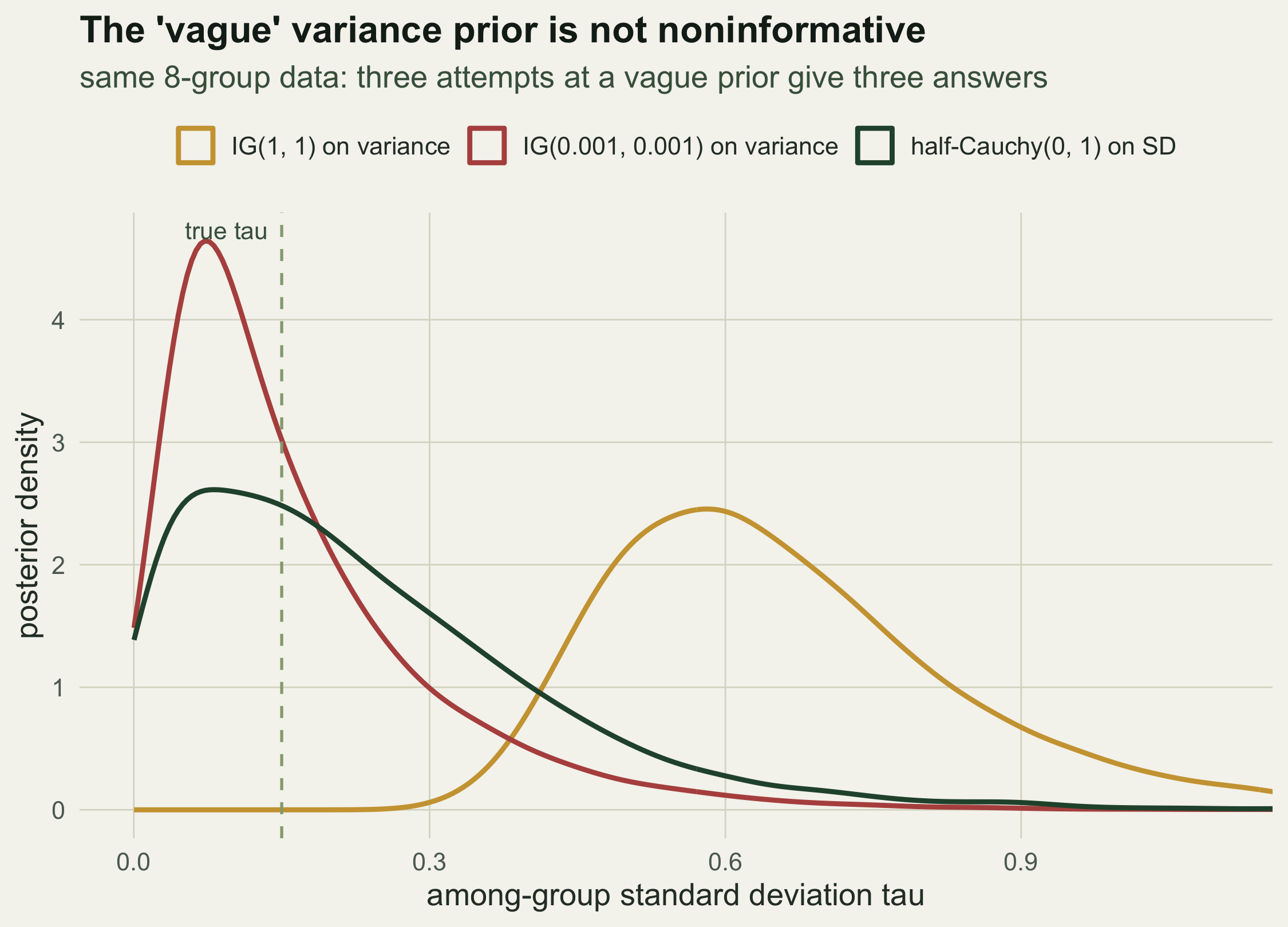
Three attempts at a vague prior, one dataset, three different answers. The inverse-gamma with parameters one has a posterior median for tau of 0.63, while shrinking the parameters to 0.001 drops the median to 0.12, a factor of 5.3 apart from what was supposed to be the same idea of ignorance. The first prior cannot let tau approach the true value at all; the second can, but only because its arbitrary parameter happened to sit in a helpful place. The half-Cauchy, the principled default from Gelman (2006), gives a median of 0.19 with a 95% interval of [0.01, 0.70] that includes values near zero, which is the honest description of data that barely constrain the spread.

lv <- c("IG(1, 1) on variance", "IG(0.001, 0.001) on variance", "half-Cauchy(0, 1) on SD")
df2 <- rbind(
  data.frame(tau = post[["IG(1, 1)"]],          prior = lv[1]),
  data.frame(tau = post[["IG(0.001, 0.001)"]],  prior = lv[2]),
  data.frame(tau = post[["half-Cauchy(0, 1)"]], prior = lv[3]))
df2$prior <- factor(df2$prior, levels = lv)
ggplot(df2, aes(tau, colour = prior)) +
  geom_density(linewidth = 1, bw = 0.035) +
  geom_vline(xintercept = tau_true, linetype = "dashed", colour = te$sage) +
  annotate("text", x = tau_true, y = Inf, label = "true tau  ", hjust = 1, vjust = 1.5,
           colour = te$label, size = 3.6) +
  scale_colour_manual(values = setNames(c(te$gold, te$terra, te$forest), lv), name = NULL) +
  coord_cartesian(xlim = c(0, 1.1)) +
  labs(x = "among-group standard deviation tau", y = "posterior density",
       title = "The 'vague' variance prior is not noninformative",
       subtitle = "same 8-group data: three attempts at a vague prior give three answers") +
  theme_te() + theme(legend.position = "top")

Figure 2: Posterior of the among-group standard deviation tau under three priors intended to be vague, on the same eight-group dataset (true tau shown dashed). The inverse-gamma priors disagree with each other and neither approaches a noninformative limit; the half-Cauchy allows tau near zero, the correct answer when the data are nearly silent about it.

What to do instead

Neither failure is an argument against priors; both are arguments for looking at what a prior implies. Two habits fix most of it. First, run prior-predictive checks: simulate parameters from the prior, generate data, and see whether that data is remotely plausible before any real data is involved (Gabry 2019). The logit example fails this check immediately. Second, when a parameter is weakly identified, do a sensitivity analysis: refit under a few reasonable priors and report whether the conclusion moves. If it does, as tau does here, that sensitivity is part of the result and should be stated, not hidden behind whichever prior gave the cleanest number.

The positive recommendation is to use weakly-informative priors on the scale that matters: a N(0, 1.5) on a logit rather than a N(0, 100), and a half-Cauchy or half-normal on a standard deviation rather than an inverse-gamma on a variance. These encode the mild, defensible knowledge that occupancy probabilities are not usually pinned at zero or one and that group differences are finite. A prior is never read on its own; it is read together with the likelihood and on the scale of the thing you care about, and “flat” is a fact about a parameterisation, not about belief.

References

• Gelman A 2006 Bayesian Analysis 1(3):515-534 (10.1214/06-BA117A)
• Northrup JM, Gerber BD 2018 PLoS ONE 13(2):e0192819 (10.1371/journal.pone.0192819)
• Gabry J, Simpson D, Vehtari A, Betancourt M, Gelman A 2019 Journal of the Royal Statistical Society A 182(2):389-402 (10.1111/rssa.12378)
• Gelman A, Carlin JB, Stern HS, Dunson DB, Vehtari A, Rubin DB 2013 Bayesian Data Analysis, 3rd edn (ISBN 978-1-4398-4095-5)
• McElreath R 2020 Statistical Rethinking, 2nd edn (ISBN 978-0-367-13991-9)

Related tutorials

• Bayesian hierarchical models with MCMC
• Single-season occupancy models
• Gibbs sampling with conjugate priors
• Logistic regression for presence-absence data