---
title: "Choosing a dissimilarity index for community data"
description: "Euclidean, Bray-Curtis, Jaccard or Hellinger: how the dissimilarity index you choose reshapes ordination of community data in R, and why double zeros matter."
date: "2026-06-25 10:00"
categories: [community ecology, multivariate, vegan, R]
image: thumbnail.png
image-alt: "Two smoothed curves of dissimilarity against gradient separation, one rising cleanly and one lagging."
---
Almost every multivariate analysis of community data starts the same way: the site-by-species table is turned into a site-by-site dissimilarity matrix, and everything downstream runs on that matrix. NMDS, PERMANOVA, hierarchical clustering and distance-based RDA all take a dissimilarity as their input. That first step looks like a formality, but it is a modelling choice. Two measures applied to the same table can rank the same pair of sites in opposite orders, and that disagreement propagates straight into the ordination.
This post works through what the common choices actually do to community data: a hand-built example that exposes the core problem, a synthetic gradient that shows it on realistic data, and the downstream effect on an ordination. The whole thing runs on `vegan`.
## The double-zero problem
Start with four species and three sites, built so the answer is obvious by eye.
```{r}
#| message: false
#| warning: false
library(vegan)

toy <- rbind(
  s1 = c(1, 1, 0, 0),
  s2 = c(0, 0, 1, 1),   # shares no species with s1
  s3 = c(4, 4, 0, 0)    # same two species as s1, higher abundance
)
colnames(toy) <- paste0("sp", 1:4)

round(as.matrix(vegdist(toy, "euclidean")), 3)
round(as.matrix(vegdist(toy, "bray")), 3)
```
Site `s1` shares both of its species with `s3` and none with `s2`. Composition says `s1` belongs next to `s3`. Euclidean distance disagrees: it makes `s1` closer to `s2` (2.000) than to `s3` (4.243). Bray-Curtis gets it right, putting `s1` next to `s3` (0.600) and as far as possible from `s2` (1.000).
The reason is the joint absences. Euclidean distance adds a squared term for every species, including the two that are absent from both `s1` and `s2`. Those shared zeros count as agreement and pull the two sites together, while the abundance gap between `s1` and `s3` inflates their distance. Bray-Curtis ignores species absent from both sites and compares the abundances they do share.
Joint absences are usually uninformative in ecology. Two sites that both lack a wetland sedge are not similar in any useful sense; they simply both sit outside its range. A dissimilarity that reads a shared absence as similarity, the way Euclidean distance does, is measuring the wrong thing. Legendre and Legendre (2012) call this the double-zero problem, and it is the single most important reason raw Euclidean distance is a poor default for species data.
## A gradient with a productivity confound
The toy is rigged, so move to something closer to field data: a coenocline of 50 sites along a moisture gradient, with 40 species placed on Gaussian niches. On top of the compositional gradient sits an independent productivity gradient, so total abundance per site varies for reasons that have nothing to do with which species are present.
```{r}
set.seed(82)
n <- 50; nsp <- 40; peak <- 26
moisture <- sort(runif(n, 0, 1))
prod <- runif(n, 0.55, 2.0)                  # productivity, independent of moisture
opt   <- seq(-0.10, 1.10, length.out = nsp)  # niche optima across the gradient
width <- runif(nsp, 0.055, 0.11)             # narrow niches give sharp turnover

lambda <- prod * outer(moisture, seq_len(nsp),
            function(m, j) peak * exp(-((m - opt[j])^2) / (2 * width[j]^2)))
comm <- matrix(rpois(n * nsp, lambda), n, nsp)
rownames(comm) <- paste0("site", seq_len(n))
colnames(comm) <- paste0("sp", seq_len(nsp))
comm <- comm[, colSums(comm) > 0]

c(sites = nrow(comm), species = ncol(comm),
  pct_zero = round(100 * mean(comm == 0), 1),
  max_abund = max(comm),
  cor_moist_prod = round(cor(moisture, prod), 2))
```
The matrix is 63% zeros, which is normal for community data: narrow niches mean most species are absent from most sites. Productivity is effectively uncorrelated with moisture (r = 0.16), so it acts as a pure nuisance: a measure that confuses abundance with composition will read it as signal.
This is the realistic version of the toy. Turnover creates double zeros between distant sites, and the productivity gradient makes total abundance vary independently of the thing we care about.
## Four measures, one question
Compute four dissimilarities and ask a simple question of each: does the distance between two sites track how far apart they sit on the moisture gradient?
```{r}
d_eu <- vegdist(comm, "euclidean")
d_bc <- vegdist(comm, "bray")
d_ja <- vegdist(comm, "jaccard", binary = TRUE)
d_he <- vegdist(decostand(comm, "hellinger"), "euclidean")  # Hellinger distance
d_grad <- dist(moisture)
```
Bray-Curtis works on abundances and ignores joint absences. Jaccard is its presence-absence sibling, built only from which species are shared. The Hellinger distance is the Euclidean distance computed after a Hellinger transformation (each row divided by its total, then square-rooted); it keeps the convenient Euclidean geometry while behaving like a composition measure, which is why it is the standard bridge to linear methods such as PCA and RDA (Legendre and Gallagher 2001).
```{r}
#| label: fig-decay
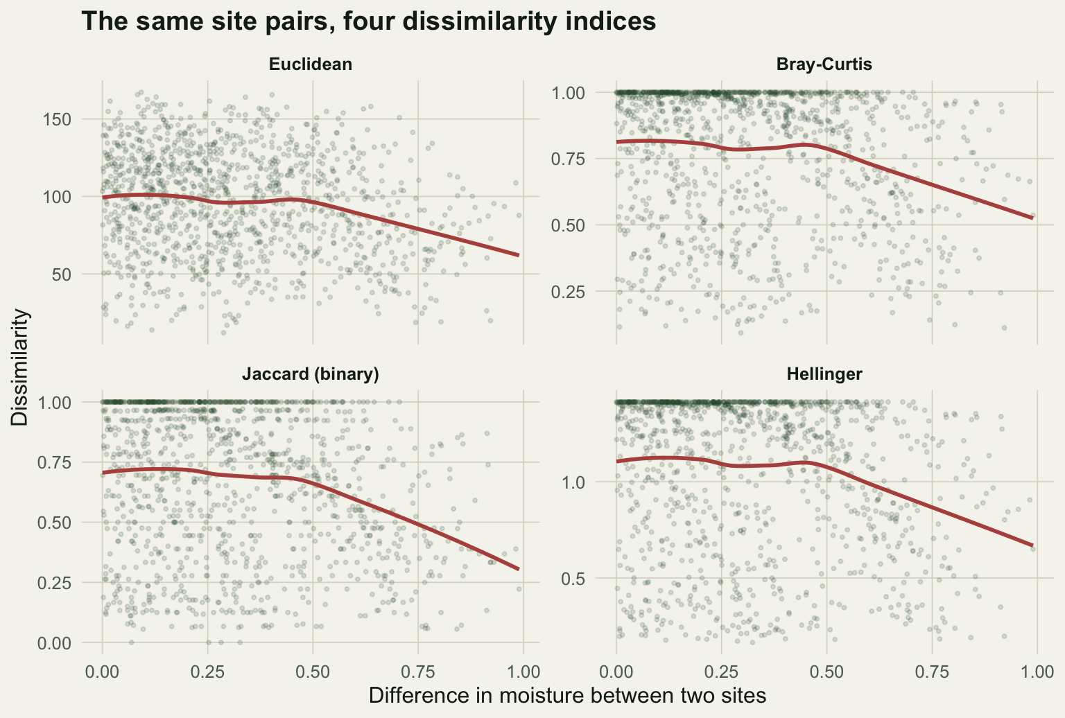
#| fig-cap: "Pairwise dissimilarity against the difference in moisture between two sites, for four indices. Each point is a site pair; the red line is a loess smoother."
#| fig-alt: "Four panels of dissimilarity versus moisture difference. Bray-Curtis, Jaccard and Hellinger form tight curves rising to a plateau; the Euclidean panel is a diffuse cloud whose smoother bends back down at large separations."
#| fig-width: 8
#| fig-height: 5.4
#| message: false
#| warning: false
library(ggplot2); library(dplyr)
pap <- "#f5f4ee"; ink <- "#16241d"; line <- "#dad9ca"
forest <- "#275139"; accent <- "#b5534e"
te_theme <- theme_minimal(base_size = 12) + theme(
  plot.background = element_rect(fill = pap, colour = NA),
  panel.background = element_rect(fill = pap, colour = NA),
  panel.grid.minor = element_blank(),
  panel.grid.major = element_line(colour = line, linewidth = .3),
  axis.title = element_text(colour = ink), axis.text = element_text(colour = "#5d6b61"),
  plot.title = element_text(colour = ink, face = "bold"),
  plot.subtitle = element_text(colour = "#5d6b61"),
  strip.text = element_text(colour = ink, face = "bold"),
  legend.title = element_text(colour = ink), legend.text = element_text(colour = "#5d6b61"))

pairs_tab <- function(dst, label) {
  m <- as.matrix(dst)
  data.frame(grad = as.vector(d_grad), dis = m[upper.tri(m)], metric = label)
}
L <- bind_rows(
  pairs_tab(d_eu, "Euclidean"), pairs_tab(d_bc, "Bray-Curtis"),
  pairs_tab(d_ja, "Jaccard (binary)"), pairs_tab(d_he, "Hellinger"))
L$metric <- factor(L$metric,
  levels = c("Euclidean", "Bray-Curtis", "Jaccard (binary)", "Hellinger"))

ggplot(L, aes(grad, dis)) +
  geom_point(alpha = .15, size = .7, colour = forest) +
  geom_smooth(method = "loess", se = FALSE, colour = accent, linewidth = 1) +
  facet_wrap(~metric, scales = "free_y") +
  labs(x = "Difference in moisture between two sites", y = "Dissimilarity",
       title = "The same site pairs, four dissimilarity indices") +
  te_theme
```
The three composition measures climb cleanly from zero and saturate once two sites stop sharing species. Raw Euclidean distance is a diffuse cloud, and its smoother bends back down at large separations: the most different pairs can look closer than moderately different ones. A Mantel correlation against gradient separation puts numbers on the pattern.
```{r}
#| message: false
#| warning: false
mant <- function(d) { set.seed(1); m <- mantel(d, d_grad, permutations = 999)
  c(r = round(m$statistic, 3), p = m$signif) }
rbind(Euclidean = mant(d_eu), `Bray-Curtis` = mant(d_bc),
      `Jaccard (binary)` = mant(d_ja), Hellinger = mant(d_he))
# how strongly does each distance track the productivity nuisance?
d_prod <- dist(prod)
c(Euclidean_vs_prod = round({ set.seed(1); mantel(d_eu, d_prod, permutations = 999)$statistic }, 2),
  Bray_vs_prod      = round({ set.seed(1); mantel(d_bc, d_prod, permutations = 999)$statistic }, 2))
```
Euclidean distance trails the field at r = 0.605, while the composition measures sit between 0.81 and 0.89. Two things drag Euclidean down. It saturates once sites share no species, so it cannot tell a large gradient gap from a very large one. And it leaks the productivity confound: Euclidean distance correlates with the difference in productivity (Mantel r = 0.15) almost twice as strongly as Bray-Curtis does (r = 0.09), because raw counts carry the abundance nuisance straight into the distance.
## The ordination inherits the distance
None of this matters in the abstract. It matters because the dissimilarity is the input to everything downstream. Run principal coordinates analysis (`cmdscale`) on each distance matrix and ask how well the first axis recovers the moisture ordering.
```{r}
#| message: false
#| warning: false
library(tidyr)
p_eu <- cmdscale(d_eu, k = 2, eig = TRUE)
p_bc <- cmdscale(d_bc, k = 2, eig = TRUE)
p_he <- cmdscale(d_he, k = 2, eig = TRUE)
rho <- function(p) abs(cor(p$points[,1], moisture, method = "spearman"))
rho_eu <- rho(p_eu); rho_bc <- rho(p_bc); rho_he <- rho(p_he)
c(Euclidean = round(rho_eu, 2), `Bray-Curtis` = round(rho_bc, 2),
  Hellinger = round(rho_he, 2),
  Bray_negeig_pct = round(100 * abs(sum(p_bc$eig[p_bc$eig < 0]) / sum(abs(p_bc$eig))), 1))
```
Bray-Curtis recovers the gradient well, Hellinger slightly better, and raw Euclidean trails. The figure shows what that means geometrically.
```{r}
#| label: fig-pcoa
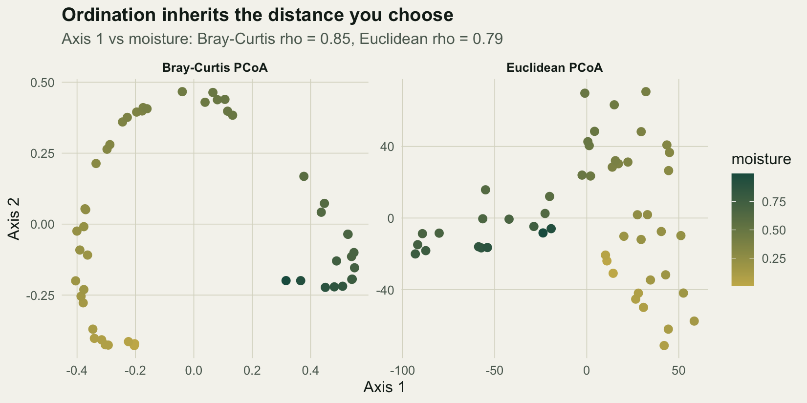
#| fig-cap: "Principal coordinates ordinations of the same community, from Euclidean and Bray-Curtis distances, with sites coloured by moisture."
#| fig-alt: "Two ordination panels coloured by moisture. The Bray-Curtis panel lays the moisture gradient as a clean arch along axis 1; the Euclidean panel folds and compresses it so high and low moisture sites mix."
#| fig-width: 8.6
#| fig-height: 4.3
#| message: false
#| warning: false
mk <- function(p, lab) data.frame(A = p$points[,1], B = p$points[,2],
                                  moisture = moisture, panel = lab)
P <- bind_rows(mk(p_bc, "Bray-Curtis PCoA"), mk(p_eu, "Euclidean PCoA"))

ggplot(P, aes(A, B, colour = moisture)) +
  geom_point(size = 2.6) +
  facet_wrap(~panel, scales = "free") +
  scale_colour_gradient(low = "#c9b458", high = "#1d5b4e", name = "moisture") +
  labs(x = "Axis 1", y = "Axis 2",
       title = "Ordination inherits the distance you choose",
       subtitle = sprintf("Axis 1 vs moisture: Bray-Curtis rho = %.2f, Euclidean rho = %.2f",
                           rho_bc, rho_eu)) +
  te_theme
```
Bray-Curtis lays the moisture gradient along the first axis as a clean arch, recovering the ordering of sites (Spearman 0.85). Euclidean distance folds the gradient and compresses the ends, so high and low moisture sites mix, and the recovery drops to 0.79. The Hellinger distance does best of all (0.87), because it strips the abundance nuisance while staying fully compatible with the Euclidean geometry that an ordination assumes.
That last point is worth holding onto. The Bray-Curtis ordination here carries 2.1% of its inertia in negative eigenvalues, the signature of a semimetric distance embedded in Euclidean space (the same issue behind the difference between `capscale` and `dbrda`). The Hellinger distance has no such problem: it is Euclidean by construction, so PCA and RDA can be run directly on Hellinger-transformed data, which is exactly how transformation-based ordination works.
## Abundance or incidence?
Bray-Curtis and Jaccard answer slightly different questions. Bray-Curtis weighs abundances; Jaccard sees only which species are shared.
```{r}
round(cor(as.vector(d_bc), as.vector(d_ja)), 2)
```
On this dataset they agree closely (correlation 0.94 between the two distance matrices), and Jaccard even edges ahead in the Mantel test. That is not a general result. Here the abundance variation is mostly productivity noise, and a presence-absence measure ignores it by construction. When abundance carries the signal, when communities shift in dominance rather than membership, Bray-Curtis sees a change that Jaccard is blind to. The choice between them is really a question about your data: is abundance signal or nuisance for the question you are asking?
## What to reach for
For abundance community data, Bray-Curtis is the sensible default, or the Hellinger distance when you want a Euclidean-embeddable measure for a linear method. For presence-absence data, Jaccard or Sorensen. Raw Euclidean distance on raw counts is the option to avoid, because it reads joint absences as similarity and conflates abundance with composition. If a method forces Euclidean geometry on you, as PCA and RDA do, transform the data first: that is precisely what the Hellinger and chord transformations are for. The dissimilarity is not a preliminary detail. It is the first model you fit, and the rest of the analysis can only be as sound as that choice.
The companion posts pick up directly from here: [NMDS ordination](../nmds-ordination/) and [PERMANOVA with envfit](../envfit-and-permanova/) both start from a Bray-Curtis matrix, [beta diversity partitioning](../beta-diversity-partitioning/) decomposes Sorensen dissimilarity, and [capscale versus dbrda](../capscale-vs-dbrda/) takes up the negative-eigenvalue problem in detail.
## References
Bray & Curtis 1957 Ecological Monographs 27(4):325-349 (10.2307/1942268)
Faith, Minchin & Belbin 1987 Vegetatio 69:57-68 (10.1007/BF00038687)
Legendre & Gallagher 2001 Oecologia 129:271-280 (10.1007/s004420100716)
Legendre & Legendre 2012 Numerical Ecology, 3rd English edition, Elsevier, Developments in Environmental Modelling 24 (ISBN 978-0-444-53868-0)