library(ggplot2)
library(dplyr)
library(tidyr)

te <- list(ink="#16241d", body="#2c3a31", forest="#275139", label="#46604a",
           sage="#93a87f", paper="#f5f4ee", line="#dad9ca", faint="#5d6b61",
           rust="#b5534e")
theme_te <- function(base_size = 11) {
  theme_minimal(base_size = base_size) +
    theme(text = element_text(colour = te$body),
          plot.title = element_text(colour = te$ink, face = "bold", size = rel(1.02)),
          plot.subtitle = element_text(colour = te$faint, size = rel(0.9)),
          axis.title = element_text(colour = te$label),
          axis.text = element_text(colour = te$faint),
          panel.grid.major = element_line(colour = te$line, linewidth = 0.3),
          panel.grid.minor = element_blank(),
          panel.background = element_rect(fill = te$paper, colour = NA),
          plot.background = element_rect(fill = te$paper, colour = NA),
          legend.key = element_rect(fill = te$paper, colour = NA),
          strip.text = element_text(colour = te$forest, face = "bold"))
}Building an integral projection model
population dynamics
demography
integral projection models
R
ecology tutorial
Build an integral projection model in R from survival, growth and fecundity regressions: assemble the kernel by the midpoint rule and read lambda from eigen.
A Leslie matrix (see Leslie matrix population models) sorts individuals into discrete age or stage classes. For many organisms the classes are awkward: a plant, a fish or a tortoise has a continuous size, and where you put the class boundaries changes the answer. The integral projection model (IPM) keeps size continuous. Instead of a matrix of class-to-class transitions it uses a kernel K(z’, z), the density of size z’ next year given size z now, built directly from regressions of survival, growth and reproduction on size.
The pay-off is that every individual informs the vital-rate functions across the whole size axis, rather than being binned into a class with a handful of neighbours. This post builds an IPM from raw individual measurements, assembles the kernel by the midpoint rule, and recovers the population growth rate lambda from the dominant eigenvalue. The numerical traps that come with the discretisation (eviction and mesh size) get their own treatment in eviction and mesh size in an IPM.
The data: individuals measured twice
An IPM needs, for a sample of marked individuals, their size z at time t and then whatever happened by t+1: did they survive, what size z’ did survivors reach, did they reproduce, and how many recruits (with what sizes) did reproducers add. Here is a synthetic perennial plant, with size on a log scale so that recruits and adults sit on the same continuous axis. The vital rates follow standard shapes: survival and flowering rise with size, growth regresses towards an equilibrium size, and recruits arrive at a small, roughly fixed size.
set.seed(4021)
n <- 2600
pars <- list(a_s=-1.4, b_s=0.50,             # survival (logit scale)
             a_g= 1.9, b_g=0.65, sig_g=0.90,  # growth (Gaussian); equilibrium 1.9/0.35
             a_f=-6.0, b_f=0.80,              # flowering probability (logit)
             a_r= 0.42, b_r=0.24,             # recruits per flowering plant (log)
             mu_r=2.2, sig_r=0.70)            # recruit size (Gaussian)

z    <- rnorm(n, 5.2, 1.9)
z    <- z[z > 0.2 & z < 11.5]; n <- length(z)
surv <- rbinom(n, 1, plogis(pars$a_s + pars$b_s * z))
zt1  <- ifelse(surv == 1, rnorm(n, pars$a_g + pars$b_g * z, pars$sig_g), NA)
flow <- rbinom(n, 1, plogis(pars$a_f + pars$b_f * z))
nrec <- ifelse(flow == 1, rpois(n, exp(pars$a_r + pars$b_r * z)), 0)
rec_sizes <- rnorm(sum(nrec), pars$mu_r, pars$sig_r)

dat <- data.frame(z = z, surv = surv, zt1 = zt1, flow = flow, nrec = nrec)
c(individuals = n, survivors = sum(surv), flowered = sum(flow), recruits = sum(nrec))
individuals survivors flowered recruits
2589 1886 578 4842 Four regressions, one per vital rate
Each vital rate is an ordinary regression on size. Survival and flowering are logistic GLMs, growth is a linear model whose residual spread gives the growth standard deviation, and recruit number is a Poisson GLM. The recruit-size distribution is summarised by its mean and standard deviation.
m_surv <- glm(surv ~ z, family = binomial, data = dat)
m_grow <- lm(zt1 ~ z, data = dat[dat$surv == 1, ])
sig_g_hat <- summary(m_grow)$sigma
m_flow <- glm(flow ~ z, family = binomial, data = dat)
m_rec  <- glm(nrec ~ z, family = poisson, data = dat[dat$flow == 1, ])
mu_r_hat  <- mean(rec_sizes); sig_r_hat <- sd(rec_sizes)

cs <- coef(m_surv); cg <- coef(m_grow); cf <- coef(m_flow); cr <- coef(m_rec)
round(rbind(survival = c(cs, NA), growth = c(cg, sigma = sig_g_hat),
            flowering = c(cf, NA), recruits = c(cr, NA)), 3)
(Intercept) z
survival -1.438 0.497 NA
growth 1.851 0.659 0.91
flowering -5.743 0.772 NA
recruits 0.313 0.254 NAThe fitted intercepts and slopes track the values used to generate the data, and the growth standard deviation comes back at 0.91 against a true 0.90. The recruit sizes centre on 2.2 with spread 0.7.
zg <- seq(0, 12, length.out = 200)
pnl <- function(d) factor(d, levels = c("Survival s(z)", "Growth z' | survived",
                                        "Flowering probability", "Recruits per flowering plant"))
pts <- bind_rows(
  transform(data.frame(z = dat$z, y = dat$surv), panel = "Survival s(z)"),
  transform(data.frame(z = dat$z[dat$surv == 1], y = dat$zt1[dat$surv == 1]), panel = "Growth z' | survived"),
  transform(data.frame(z = dat$z, y = dat$flow), panel = "Flowering probability"),
  transform(data.frame(z = dat$z[dat$flow == 1], y = dat$nrec[dat$flow == 1]), panel = "Recruits per flowering plant"))
pts$panel <- pnl(pts$panel)
lns <- bind_rows(
  transform(data.frame(z = zg, y = plogis(cs[1] + cs[2] * zg)), panel = "Survival s(z)"),
  transform(data.frame(z = zg, y = cg[1] + cg[2] * zg), panel = "Growth z' | survived"),
  transform(data.frame(z = zg, y = plogis(cf[1] + cf[2] * zg)), panel = "Flowering probability"),
  transform(data.frame(z = zg, y = exp(cr[1] + cr[2] * zg)), panel = "Recruits per flowering plant"))
lns$panel <- pnl(lns$panel)

ggplot() +
  geom_point(data = pts, aes(z, y), colour = te$sage, alpha = 0.28, size = 0.7,
             position = position_jitter(height = 0.02, width = 0)) +
  geom_abline(data = data.frame(panel = pnl("Growth z' | survived")),
              aes(slope = 1, intercept = 0), linetype = "dashed", colour = te$faint, linewidth = 0.35) +
  geom_line(data = lns, aes(z, y), colour = te$rust, linewidth = 0.9) +
  facet_wrap(~panel, scales = "free_y") +
  labs(x = "Size z at time t (log scale)", y = NULL) +
  theme_te(11)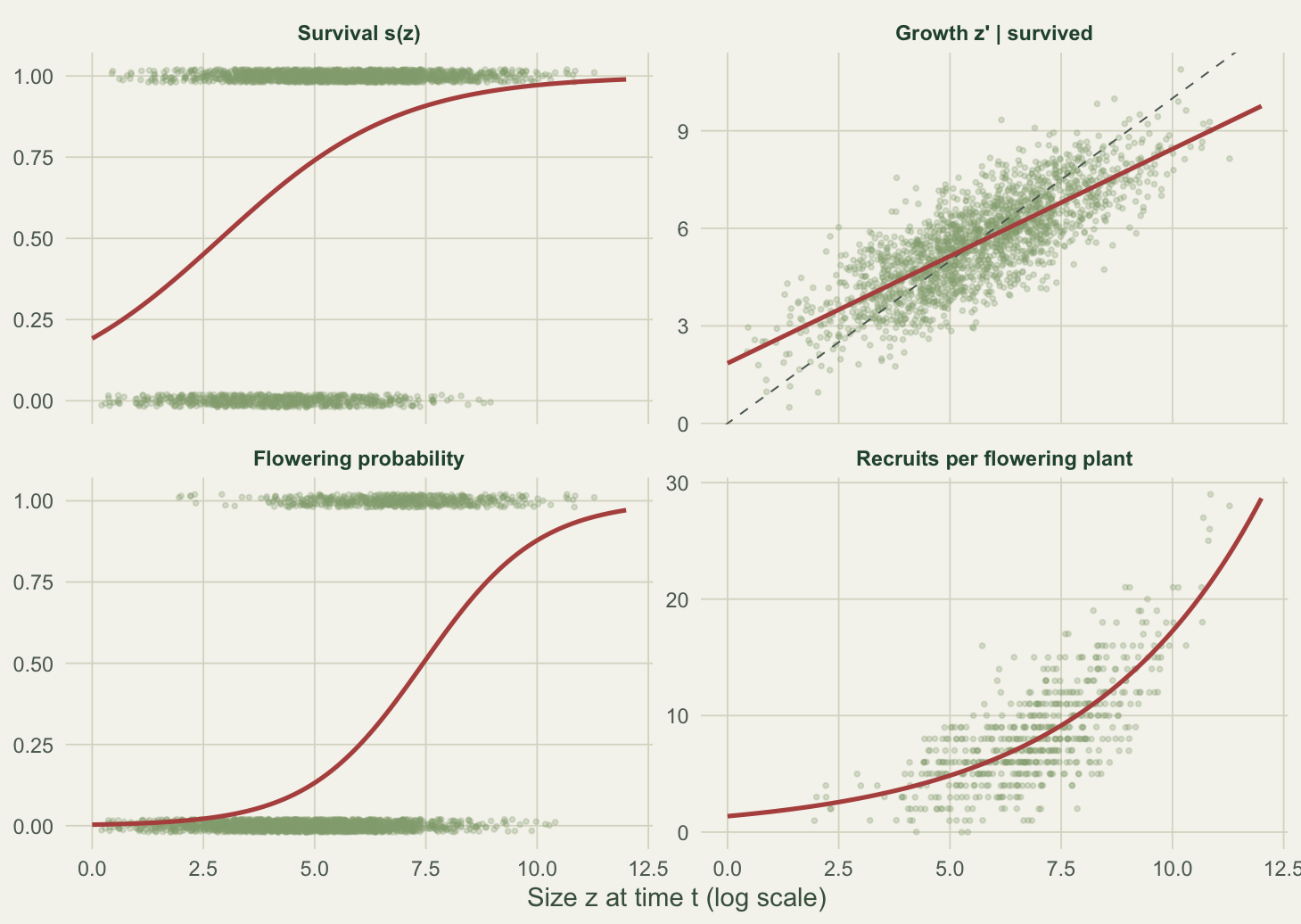
Assembling the kernel by the midpoint rule
The kernel splits into two parts. The survival-growth part moves existing plants:
P(z’, z) = s(z) G(z’, z),
where s(z) is survival and G(z’, z) is the growth density (a Gaussian centred on the fitted growth line). The fecundity part adds recruits:
F(z’, z) = p_f(z) R(z) C(z’),
where p_f is the flowering probability, R is the expected number of recruits, and C(z’) is the recruit-size density. The full kernel is K = P + F.
To turn this continuous operator into something you can eigen-analyse, apply the midpoint rule: lay a mesh of m points across the size range, evaluate the kernel at every pair of midpoints, and multiply by the bin width h. The kernel becomes an m by m matrix, and from there the machinery is identical to a matrix model: lambda is the dominant eigenvalue.
build_K <- function(cs, cg, sig_g, cf, cr, mu_r, sig_r, L, U, m) {
  h    <- (U - L) / m
  mesh <- L + (1:m - 0.5) * h                                   # bin midpoints
  S  <- plogis(cs[1] + cs[2] * mesh)                            # survival at each z
  G  <- outer(mesh, mesh, function(zp, z) dnorm(zp, cg[1] + cg[2] * z, sig_g))
  P  <- sweep(G, 2, S, "*") * h                                 # survival-growth
  Pf <- plogis(cf[1] + cf[2] * mesh)                            # flowering probability
  Rn <- exp(cr[1] + cr[2] * mesh)                               # expected recruits
  Cr <- dnorm(mesh, mu_r, sig_r)                                # recruit-size density
  Fk <- outer(Cr, Pf * Rn) * h                                  # fecundity
  list(K = P + Fk, mesh = mesh, h = h, S = S, colP = colSums(P))
}

L <- 0; U <- 12; m <- 100
fit    <- build_K(cs, cg, sig_g_hat, cf, cr, mu_r_hat, sig_r_hat, L, U, m)
ev     <- eigen(fit$K)
lambda <- Re(ev$values[1])
w      <- Re(ev$vectors[, 1]); w <- w / sum(w)                  # stable size distribution
lambda
[1] 1.007045The mesh runs from 0 to 12 on the log-size scale with m = 100 bins, so the bin width is h = 0.12. The dominant eigenvalue is lambda = 1.007, a population growing slowly.
kdf <- data.frame(z = rep(fit$mesh, each = m), zp = rep(fit$mesh, times = m),
                  val = as.vector(fit$K))
ggplot(kdf, aes(z, zp, fill = val)) +
  geom_raster(interpolate = TRUE) +
  geom_abline(slope = 1, intercept = 0, linetype = "dashed", colour = "#ffffffaa", linewidth = 0.4) +
  scale_fill_gradient(low = te$paper, high = te$forest, trans = "sqrt", name = "K(z', z)") +
  coord_equal(expand = FALSE) +
  labs(x = "Size z at time t", y = "Size z' at time t+1") +
  theme_te(11) + theme(panel.grid = element_blank())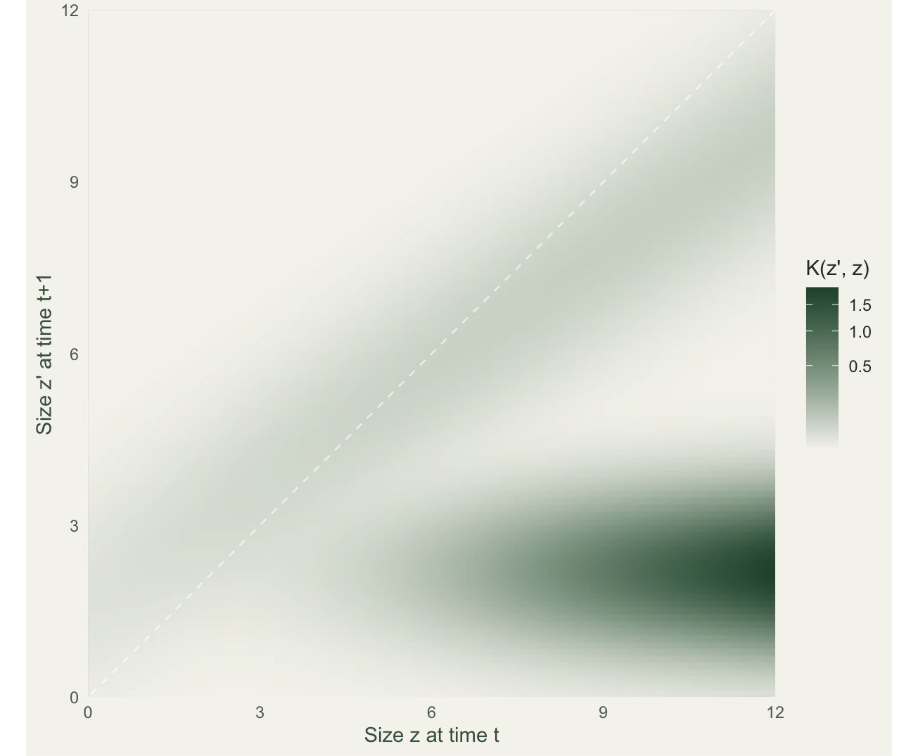
Does it recover the truth?
Because this is synthetic data, the true growth rate is known: build the same kernel from the generating parameters on the same mesh and take its dominant eigenvalue. Any gap between the two is sampling error in the vital-rate fits, not a difference of method.
tru <- build_K(c(pars$a_s, pars$b_s), c(pars$a_g, pars$b_g), pars$sig_g,
               c(pars$a_f, pars$b_f), c(pars$a_r, pars$b_r), pars$mu_r, pars$sig_r, L, U, m)
lambda_true <- Re(eigen(tru$K)$values[1])
c(fitted = lambda, true = lambda_true, difference = lambda - lambda_true)
fitted true difference
1.0070446 1.0131351 -0.0060905 The fitted IPM lands at lambda = 1.007 against the true 1.013, a gap of 0.6 per cent. The individual coefficients each carry their own noise (the recruit intercept, for instance, is estimated a little low), but lambda is an emergent quantity and the errors partly cancel.
One more contrast is worth drawing. The dominant right eigenvector is the stable size distribution, the shape the population settles into. Its mean size is 3.44, well below the mean of the sampled plants (5.23). The two differ because the sample was drawn across the size range for fitting, whereas the stable distribution is dominated by the many small recruits that high fecundity produces. The observed size distribution is not the stable one, exactly as the observed age distribution is not the stable age distribution in a Leslie model.
What the kernel buys you, and what to check next
The IPM turns a set of one-variable regressions into a projection operator without ever choosing a class boundary. Growth, survival and fecundity can each be modelled with the tools you already use (GLM, GAM, mixed models), and the kernel inherits their smoothness. That is the strength: the size dependence is estimated once, from all the data, rather than assumed piecewise.
The weakness is that the eigen-analysis runs on a discretised approximation, and the midpoint rule has two failure modes. A Gaussian growth density on a bounded mesh loses probability mass off the edges, so plants are quietly evicted and lambda drifts low; and too coarse a mesh under-resolves the kernel. Here both were kept small (the mesh amply covers the data, and the largest missing survival mass at the edge is under 0.006), but neither is automatic. Checking them is the subject of the next post.
References
Easterling MR, Ellner SP, Dixon PM 2000. Ecology 81(3):694-708 (10.1890/0012-9658(2000)081[0694:SSSAAN]2.0.CO;2).
Ellner SP, Rees M 2006. American Naturalist 167(3):410-428 (10.1086/499438).
Merow C, Dahlgren JP, Metcalf CJE, Childs DZ, Evans MEK, Jongejans E, Record S, Rees M, Salguero-Gomez R, McMahon SM 2014. Methods in Ecology and Evolution 5(2):99-110 (10.1111/2041-210X.12146).
Rees M, Childs DZ, Ellner SP 2014. Journal of Animal Ecology 83(3):528-545 (10.1111/1365-2656.12178).
Coulson T 2012. Oikos 121(9):1337-1350 (10.1111/j.1600-0706.2012.00035.x).
Ellner SP, Childs DZ, Rees M 2016. Data-driven Modelling of Structured Populations. Springer. ISBN 978-3-319-28891-8.