library(ggplot2)
library(patchwork)

te_paper  <- "#f5f4ee"
te_ink    <- "#16241d"
te_body   <- "#2c3a31"
te_forest <- "#275139"
te_rust   <- "#b5534e"
te_gold   <- "#c9b458"
te_line   <- "#dad9ca"

theme_datasheet <- function() {
  theme_minimal(base_size = 12) +
    theme(plot.background  = element_rect(fill = te_paper, colour = NA),
          panel.background = element_rect(fill = te_paper, colour = NA),
          panel.grid.major = element_line(colour = te_line, linewidth = 0.3),
          panel.grid.minor = element_blank(),
          text             = element_text(colour = te_body),
          plot.title       = element_text(colour = te_ink, face = "bold"),
          plot.subtitle    = element_text(colour = te_body),
          axis.text        = element_text(colour = te_body))
}Quadrat variance peaks and false second scales
R
spatial pattern
quadrat variance
statistics
ecology tutorial
TTLQV and paired quadrat variance on transects with one patch scale: how often a second peak appears, where it lands, and why a peak count is not a scale count.
A student has laid a line of one thousand contiguous 10 cm quadrats across a grassland slope and scored the cover of a clonal sedge in each one. The sedge grows in patches with bare ground between them, and the question is the size of the patches. The textbook tool is a blocked quadrat variance: combine neighbouring quadrats into blocks of increasing size, compare adjacent blocks, and plot the variance against block size. A peak marks a scale of pattern. The student’s curve has a clear peak near a metre, and then a second, lower peak near three metres. The report says the sedge is patchy at two scales, one of clumps and one of clusters of clumps.
That reading is the subject of this post. The two quadrat variance methods used here come from the vegetation literature of the 1970s: two-term local quadrat variance (TTLQV), set out by Hill, and paired quadrat variance (PQV), compared with the blocked methods by Ludwig and Goodall. Both are still in use for belt transects of cover, and both are simple enough to write in a dozen lines of base R. The simulations below build transects with exactly one patch scale, with patch and gap widths that range from perfectly regular to very irregular, and count how often the rule “each peak is a scale” reports a second scale that was never put there.
The wavelet posts on this site cover a neighbouring problem. Wavelet significance and the red noise null asks whether a patch of wavelet power is bigger than the patches noise makes, and checking a wavelet analysis shows real features read as the wrong structure in a time series. The question here comes before significance: one scale of pattern gives a quadrat variance curve with more than one peak. For point patterns the same job of reading a scale from a curve falls to Ripley’s K and the pair correlation function.
Two variances and one peak rule
Write the cover in quadrat i as x_i, for i from 1 to n. For a block size b, TTLQV slides a window of two adjacent blocks of b quadrats along the transect, takes the difference between the two block totals, squares it, and averages:
V2(b) = sum over i from 1 to n + 1 - 2b of (x_i + … + x_(i+b-1) - x_(i+b) - … - x_(i+2b-1))^2, divided by 2b(n + 1 - 2b).
The divisor 2b makes the value for unpatterned data with variance s^2 equal to s^2 at every block size. PQV compares single quadrats b apart instead of blocks, and is the semivariogram of the transect at lag b:
P(b) = sum over i from 1 to n - b of (x_i - x_(i+b))^2, divided by 2(n - b).
At b = 1 the two are the same number. Both are computed below with cumulative sums, one vectorised pass per block size.
The peak rule has to be fixed before any curve is looked at, and it has to be the same for both methods. A block size counts as a peak when its value is the strict maximum within two block sizes either side, and when it stands above the lowest point of the curve since the previous accepted peak (or since b = 1) by at least a fixed fraction of its own height. That fraction is the margin. The primary margin is one tenth; the rates are also reported at one twentieth and one fifth, because the answer moves with it and a reader should see how much. Block sizes run to 100, one tenth of the transect: the formulas allow larger blocks, but the largest ones rest on very few independent comparisons.
n_quad    <- 1000
w_mean    <- 10
b_max     <- 100
noise_sd  <- 0.5
win_half  <- 2
agree_tol <- 3
margins   <- c(0.05, 0.10, 0.20)
m_main    <- 0.10

ttlqv <- function(x, bmax) {
  n_x   <- length(x)
  cum_x <- c(0, cumsum(x))
  vapply(seq_len(bmax), function(b) {
    i_start <- seq_len(n_x + 1 - 2 * b)
    left  <- cum_x[i_start + b] - cum_x[i_start]
    right <- cum_x[i_start + 2 * b] - cum_x[i_start + b]
    sum((left - right)^2) / (2 * b * (n_x + 1 - 2 * b))
  }, numeric(1))
}

pqv <- function(x, bmax) {
  n_x <- length(x)
  vapply(seq_len(bmax), function(b) {
    sum((x[1:(n_x - b)] - x[(1 + b):n_x])^2) / (2 * (n_x - b))
  }, numeric(1))
}

find_peaks <- function(v, margin, half = win_half) {
  n_b  <- length(v)
  mid  <- (1 + half):(n_b - half)
  win  <- sapply(-half:half, function(k) v[mid + k])
  cand <- mid[v[mid] == apply(win, 1, max) & rowSums(win == v[mid]) == 1]
  peaks  <- integer(0)
  last_b <- 1
  for (b in cand) {
    if (v[b] - min(v[last_b:b]) >= margin * v[b]) {
      peaks  <- c(peaks, b)
      last_b <- b
    }
  }
  peaks
}

make_transect <- function(n, w, cv, sd_noise) {
  draw_w <- function(k) {
    if (cv == 0) return(rep(w, k))
    pmax(1, round(rgamma(k, shape = 1 / cv^2, scale = w * cv^2)))
  }
  k_run  <- ceiling(2 * n / w) + 50
  runs   <- as.vector(rbind(draw_w(k_run), draw_w(k_run)))
  cover  <- rep(rep(c(0, 1), k_run), runs)
  offset <- sample.int(2 * w, 1)
  cover[offset:(offset + n - 1)] + rnorm(n, 0, sd_noise)
}
The transects alternate gaps of cover 0 and patches of cover 1, with widths drawn from a gamma distribution of mean 10 quadrats and a chosen coefficient of variation (CV), rounded to whole quadrats; gaps and patches have the same distribution, so the pattern has one scale. Gaussian noise with a standard deviation of 0.5 is added to every quadrat, and the start of the transect falls at a random point in the first cycle. All of these constants, the margins included, were set before the replicate runs; a small pilot was used only to check that the code ran and how long it took.
One scale, a row of peaks: the square wave
square_x <- rep(rep(c(1, 0), each = w_mean), n_quad / (2 * w_mean))
sq_t <- ttlqv(square_x, b_max)
sq_p <- pqv(square_x, b_max)
pk_sq_t <- find_peaks(sq_t, m_main)
pk_sq_p <- find_peaks(sq_p, m_main)
ratio_t3 <- sq_t[pk_sq_t[2]] / sq_t[pk_sq_t[1]]
ratio_t5 <- sq_t[pk_sq_t[3]] / sq_t[pk_sq_t[1]]
ratio_p3 <- sq_p[pk_sq_p[2]] / sq_p[pk_sq_p[1]]
ratio_t3_noise <- (sq_t[pk_sq_t[2]] + noise_sd^2) / (sq_t[pk_sq_t[1]] + noise_sd^2)

big_w    <- 200
big_x    <- rep(rep(c(1, 0), each = big_w), 10)
big_peak <- which.max(ttlqv(big_x, round(1.2 * big_w))) / big_w
Start with no randomness at all: patches and gaps of exactly 10 quadrats, no noise. TTLQV has peaks at block sizes 9, 30, 50, 70, 90, and PQV at 10, 30, 50, 70, 90. The first TTLQV peak sits one quadrat below the patch width; on a much coarser square wave, with patches of 200 quadrats, it sits at 0.89 of the patch width, so this is a property of TTLQV and not of rounding. The usual reading, that the TTLQV peak falls near the patch size when patches and gaps are equal (Guo and Kelly report it for transects with equal mean patch and gap sizes), holds in that sense: near, and a little below.
The later peaks are the pattern repeating. A pair of blocks of three patch widths each covers one and a half cycles on each side, and the two block totals differ by exactly one patch width, the same difference as at the true scale. TTLQV divides by 2b, so the peak at three widths has 0.317 of the height of the first, and the one at five widths 0.190: close to one third and one fifth. PQV has no such divisor. Quadrats three patch widths apart are always on opposite phases, exactly as at one width, and its second peak is 1.000 times the first. On a regular pattern both methods therefore put the extra peaks at the same odd multiples of the patch width. They do not disagree.
sq_df <- data.frame(b = rep(seq_len(b_max), 2),
                    value = c(sq_t / max(sq_t), sq_p / max(sq_p)),
                    method = rep(c("TTLQV", "PQV"), each = b_max))
ggplot(sq_df, aes(b, value, colour = method)) +
  geom_vline(xintercept = w_mean * c(1, 3, 5, 7, 9), linetype = "dashed",
             colour = te_line, linewidth = 0.6) +
  geom_line(linewidth = 0.9) +
  scale_colour_manual(values = c(TTLQV = te_forest, PQV = te_rust), name = NULL) +
  scale_x_continuous(breaks = seq(0, b_max, by = 10)) +
  labs(x = "block size or lag (quadrats)", y = "variance / its maximum",
       title = "One patch width, five peaks",
       subtitle = "dashed: odd multiples of the patch width") +
  theme_datasheet() +
  theme(legend.position = "bottom")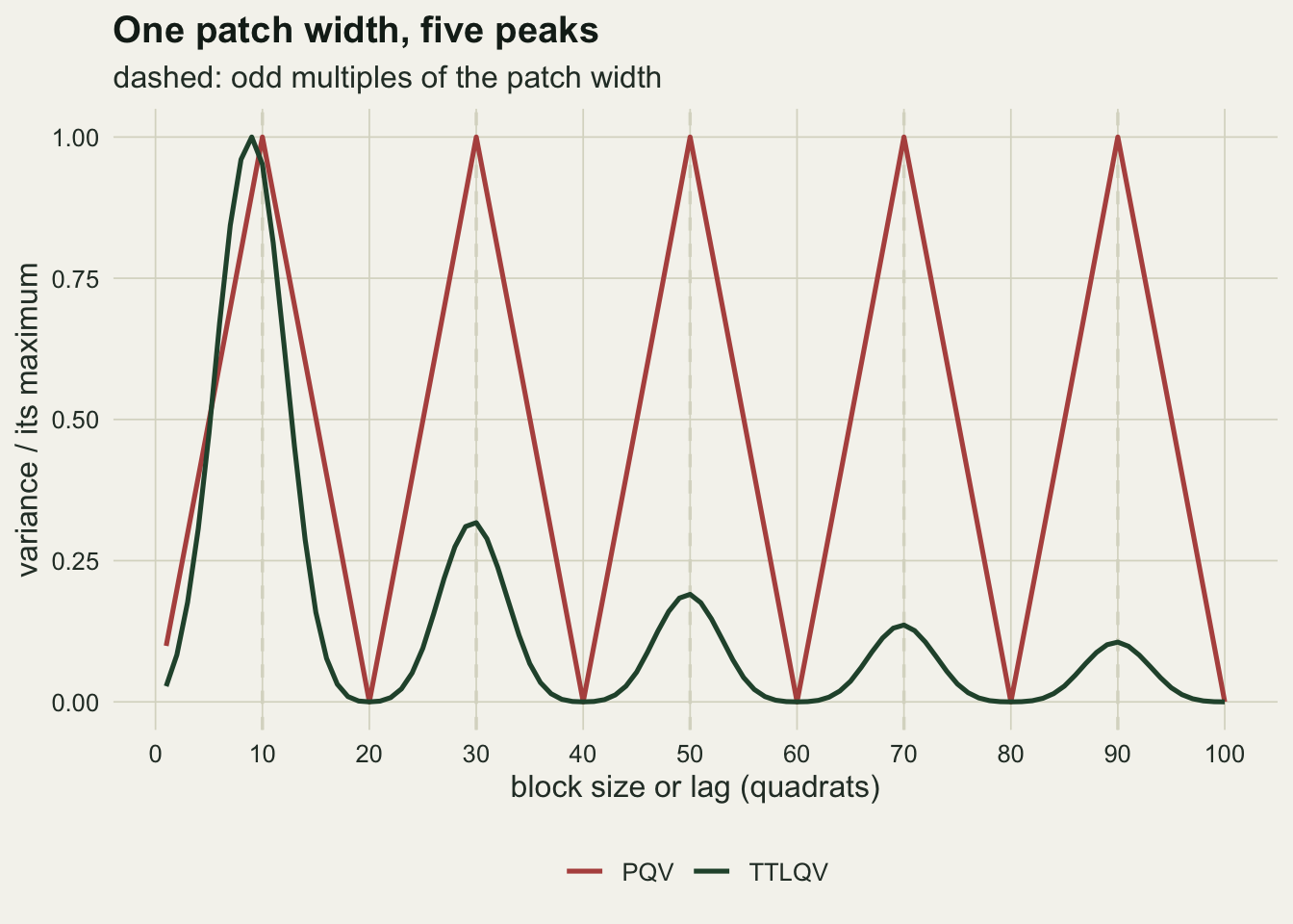
An irregular transect, and a shuffled null
set.seed(2718)
one_x <- make_transect(n_quad, w_mean, 0.4, noise_sd)
one_t <- ttlqv(one_x, b_max)
one_p <- pqv(one_x, b_max)
pk_one_t <- find_peaks(one_t, m_main)
pk_one_p <- find_peaks(one_p, m_main)

n_shuffle <- 499
null_curves <- replicate(n_shuffle, {
  shuffled <- sample(one_x)
  c(ttlqv(shuffled, b_max), pqv(shuffled, b_max)) / var(one_x)
})
env_t <- apply(null_curves[1:b_max, ], 1, quantile, probs = 0.95)
env_p <- apply(null_curves[b_max + 1:b_max, ], 1, quantile, probs = 0.95)
one_scaled_t <- one_t / var(one_x)
one_scaled_p <- one_p / var(one_x)
env_mean_t <- mean(null_curves[1:b_max, ])
over_t <- one_scaled_t[pk_one_t] > env_t[pk_one_t]
over_p <- one_scaled_p[pk_one_p] > env_p[pk_one_p]
env_ends_t <- env_t[c(20, b_max)]

b_idx <- 20:b_max
lag1_cor <- function(block) {
  mean(apply(block[b_idx, ], 2, function(z) cor(z[-1], z[-length(z)])))
}
nb_cor_t <- lag1_cor(null_curves[1:b_max, ])
nb_cor_p <- lag1_cor(null_curves[b_max + 1:b_max, ])
n_cand_t <- mean(apply(null_curves[1:b_max, ], 2, function(v) length(find_peaks(v, 0))))
n_cand_p <- mean(apply(null_curves[b_max + 1:b_max, ], 2, function(v) length(find_peaks(v, 0))))
rel_sd_t <- apply(null_curves[1:b_max, ], 1, sd)[50] / mean(null_curves[50, ])
rel_sd_p <- apply(null_curves[b_max + 1:b_max, ], 1, sd)[50] / mean(null_curves[b_max + 50, ])
A single transect with a CV of 0.4 in the patch and gap widths looks more like field data. TTLQV accepts 1 peak (at block size 9) and PQV accepts 4, at 9, 26, 36, 53. Two methods on the same quadrats, one scale in the simulation, and two different counts. The obvious next step is a null: shuffle the quadrats, which destroys every spatial pattern and keeps the values, and see where the curves of 499 shuffled transects lie. Scaled by the transect variance, the shuffled curves average 1.017 for TTLQV, as the divisor promises. Their pointwise 95 per cent line is not flat, though: for TTLQV it rises, unevenly, from 1.31 at block size 20 to 1.75 at 100, because large blocks give few independent differences.
Of the TTLQV peaks on this transect, 1 of 1 clear the pointwise line; of the PQV peaks, 2 of 4 do. This is a pointwise version of the check the wavelet posts ask for, and the replicate section below measures how often a second peak clears it.
strip_df <- data.frame(quadrat = seq_len(n_quad), cover = one_x)
p_strip <- ggplot(strip_df[1:300, ], aes(quadrat, cover)) +
  geom_line(colour = te_body, linewidth = 0.35) +
  labs(x = "quadrat (first 300 of 1000)", y = "cover",
       title = "Irregular patches, one scale") +
  theme_datasheet()
curve_df <- data.frame(b = rep(seq_len(b_max), 2),
                       value = c(one_scaled_t, one_scaled_p),
                       envelope = c(env_t, env_p),
                       method = rep(c("TTLQV", "PQV"), each = b_max))
curve_df$method <- factor(curve_df$method, levels = c("TTLQV", "PQV"))
peak_df <- data.frame(b = c(pk_one_t, pk_one_p),
                      value = c(one_scaled_t[pk_one_t], one_scaled_p[pk_one_p]),
                      method = factor(rep(c("TTLQV", "PQV"),
                                          c(length(pk_one_t), length(pk_one_p))),
                                      levels = c("TTLQV", "PQV")))
p_curves <- ggplot(curve_df, aes(b, value)) +
  geom_line(aes(y = envelope), colour = te_gold, linewidth = 0.8, linetype = "dashed") +
  geom_line(colour = te_forest, linewidth = 0.9) +
  geom_point(data = peak_df, colour = te_rust, size = 2.6) +
  facet_wrap(~ method, ncol = 2, scales = "free_y") +
  labs(x = "block size or lag (quadrats)", y = "variance / transect variance",
       subtitle = "red points: accepted peaks; dashed gold: 95 per cent of shuffled transects") +
  theme_datasheet()
p_strip / p_curves + plot_layout(heights = c(1, 1.6)) +
  plot_annotation(theme = theme_datasheet())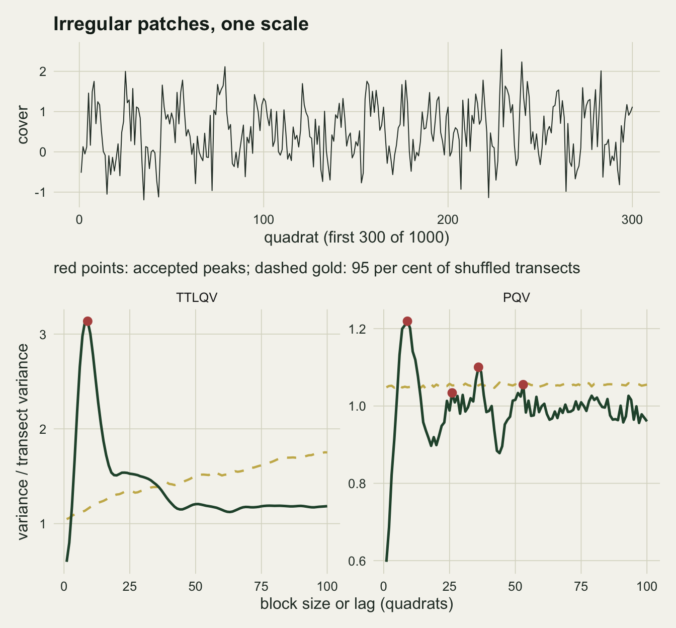
How often a second peak appears
cv_grid <- c(0, 0.2, 0.4, 0.7, 1)
n_rep   <- 500

null_q_t <- env_t
null_q_p <- env_p

curve_summary <- function(v, v_scale, env) {
  n_by_margin <- vapply(margins, function(m) length(find_peaks(v, m)), numeric(1))
  pk <- c(find_peaks(v, m_main), NA, NA)[1:2]
  c(n_by_margin, pk, v[pk[2]] / v[pk[1]], v[pk[2]] / v_scale > env[pk[2]])
}

run_condition <- function(gen, label) {
  res <- t(replicate(n_rep, {
    x <- gen()
    c(curve_summary(ttlqv(x, b_max), var(x), null_q_t),
      curve_summary(pqv(x, b_max), var(x), null_q_p))
  }))
  cols <- c("n05", "n10", "n20", "first", "second", "height_ratio", "over_null")
  out_t <- as.data.frame(res[, 1:7]);  names(out_t) <- cols
  out_p <- as.data.frame(res[, 8:14]); names(out_p) <- cols
  rbind(data.frame(condition = label, rep = seq_len(n_rep), method = "TTLQV", out_t),
        data.frame(condition = label, rep = seq_len(n_rep), method = "PQV", out_p))
}

set.seed(3107)
sim_all <- do.call(rbind, c(
  lapply(cv_grid, function(cv)
    run_condition(function() make_transect(n_quad, w_mean, cv, noise_sd),
                  sprintf("CV %.1f", cv))),
  list(run_condition(function() rnorm(n_quad, 0.5, noise_sd), "no pattern"))))
cond_levels <- c(sprintf("CV %.1f", cv_grid), "no pattern")
sim_all$condition <- factor(sim_all$condition, levels = cond_levels)

rate_of <- function(cond, meth, col) {
  z <- sim_all[sim_all$condition == cond & sim_all$method == meth, col]
  mean(z >= 2)
}
rate_tab <- expand.grid(condition = cond_levels, method = c("TTLQV", "PQV"),
                        margin = margins, stringsAsFactors = FALSE)
rate_tab$col  <- c("n05", "n10", "n20")[match(rate_tab$margin, margins)]
rate_tab$rate <- mapply(rate_of, rate_tab$condition, rate_tab$method, rate_tab$col)
rate_tab$se   <- sqrt(rate_tab$rate * (1 - rate_tab$rate) / n_rep)
get_rate <- function(cond, meth, m = m_main) {
  rate_tab$rate[rate_tab$condition == cond & rate_tab$method == meth & rate_tab$margin == m]
}
max_se <- max(rate_tab$se)

set.seed(3108)
strict_m <- c(0.3, 0.5)
n_strict <- 200
strict_hits <- replicate(n_strict, {
  x <- make_transect(n_quad, w_mean, 0.2, noise_sd)
  c(vapply(strict_m, function(m) length(find_peaks(ttlqv(x, b_max), m)) >= 2, logical(1)),
    vapply(strict_m, function(m) length(find_peaks(pqv(x, b_max), m)) >= 2, logical(1)))
})
strict_rate_t <- rowMeans(strict_hits)[1:2]
strict_rate_p <- rowMeans(strict_hits)[3:4]
Each of five CV values, from a regular pattern to widths as variable as an exponential distribution, got 500 transects, and so did a sixth condition with no pattern at all: noise around a constant cover. With a rate of one half, 500 transects give a Monte Carlo standard error of 0.022; the largest standard error in the table is 0.022.
At the primary margin, a transect with a CV of 0.2 shows at least two TTLQV peaks in 100.0 per cent of runs and at least two PQV peaks in 100.0 per cent. At a CV of 0.4 the TTLQV rate is 70.4 per cent, at 0.7 it is 48.2 per cent, and at 1 it is 17.4 per cent. PQV stays at 99.0 per cent even at a CV of 1.
The no-pattern row explains most of the PQV figure and part of the TTLQV one. Pure noise gives two or more TTLQV peaks in 40.6 per cent of transects and two or more PQV peaks in 98.2 per cent. The reason is in how the two curves are built, not in the margin being unfair to PQV. PQV at neighbouring lags uses almost independent pairs of quadrats, so a noise curve jumps from lag to lag, while TTLQV at neighbouring block sizes shares nearly all its quadrats and moves smoothly. Over block sizes 20 to 100 of the shuffled curves above, the correlation between the deviations at neighbouring block sizes averages 0.996 for TTLQV and -0.001 for PQV, and the window rule alone, before any margin and over the whole curve, finds on average 3.9 local maxima on a shuffled TTLQV curve and 19.2 on a shuffled PQV curve. With that many candidates, one standing a tenth above the dip before it is almost always there. At a margin of one fifth the noise rates fall to 5.8 per cent for TTLQV and 0.0 per cent for PQV, while a CV of 0.2 still gives 99.4 and 100.0 per cent. The second peak of a near-regular pattern survives a margin of one fifth and the second peak of noise does not, but it is not indestructible: in a further 200 transects with a CV of 0.2, a margin of 0.3 leaves two or more peaks in 93.5 per cent for TTLQV and 100.0 per cent for PQV, and a margin of one half in only 11.0 and 2.5 per cent. A strict enough margin removes the harmonic along with the noise, and with it any second scale of similar prominence.
rate_tab$condition <- factor(rate_tab$condition, levels = cond_levels)
rate_tab$margin_lab <- factor(sprintf("margin %.2f", rate_tab$margin))
rate_tab$method <- factor(rate_tab$method, levels = c("TTLQV", "PQV"))
ggplot(rate_tab, aes(condition, rate, colour = margin_lab, group = margin_lab)) +
  geom_line(linewidth = 0.8) +
  geom_point(size = 2.4) +
  facet_wrap(~ method, ncol = 2) +
  scale_colour_manual(values = c(te_gold, te_forest, te_rust), name = NULL) +
  scale_y_continuous(limits = c(0, 1)) +
  labs(x = NULL, y = "share with two or more peaks",
       title = "Second peaks are common, and noise makes them too",
       subtitle = "single-scale transects; last column: noise with no pattern") +
  theme_datasheet() +
  theme(legend.position = "bottom",
        axis.text.x = element_text(angle = 35, hjust = 1))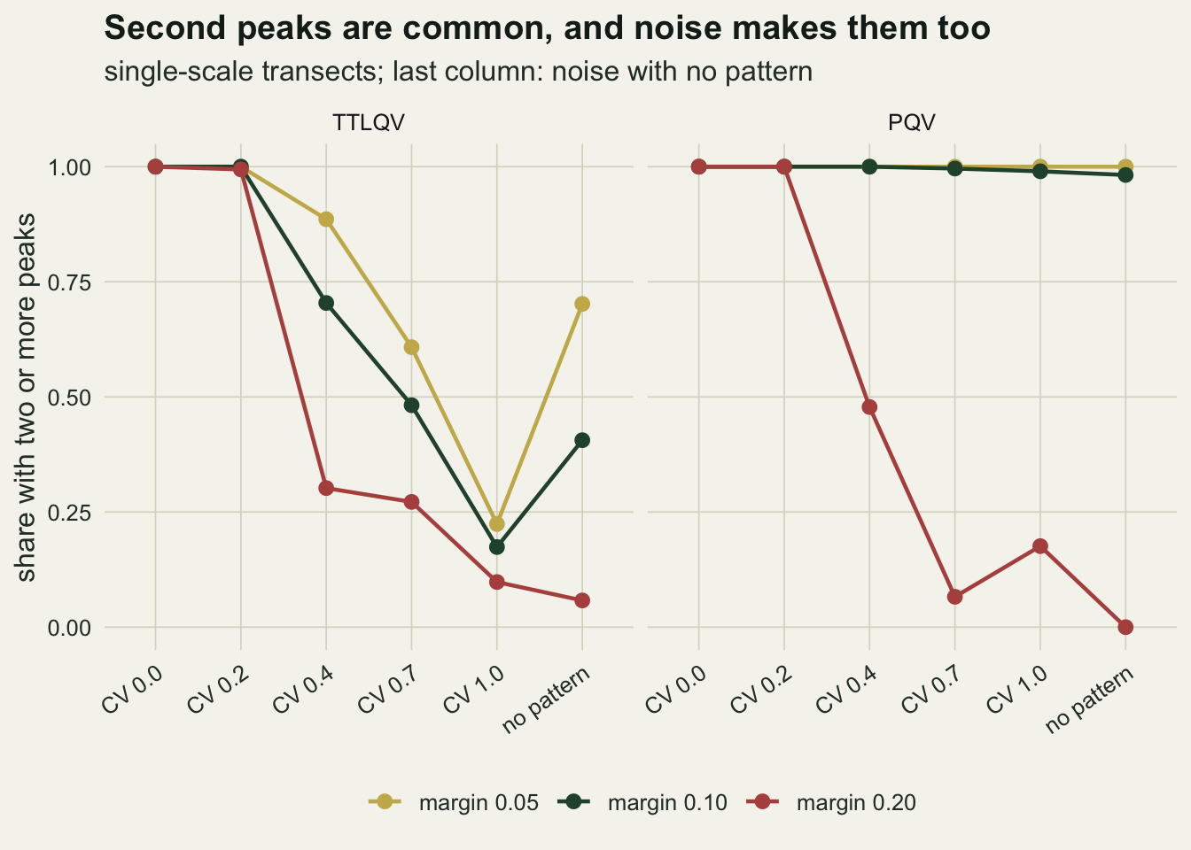
Where the second peak lands, and whether the methods agree
m_sub <- sim_all[!is.na(sim_all$second), ]
m_sub$second_w <- m_sub$second / w_mean
m_sub$ratio    <- m_sub$second / m_sub$first

loc_q <- function(cond, meth, p) {
  quantile(m_sub$second_w[m_sub$condition == cond & m_sub$method == meth], p, names = FALSE)
}
near_three <- function(cond, meth) {
  z <- m_sub$ratio[m_sub$condition == cond & m_sub$method == meth]
  mean(abs(z - 3) <= 0.5)
}
height_q <- function(cond, p) {
  quantile(m_sub$height_ratio[m_sub$condition == cond & m_sub$method == "TTLQV"], p, names = FALSE)
}
over_rate <- function(cond, meth) {
  mean(m_sub$over_null[m_sub$condition == cond & m_sub$method == meth] == 1)
}

tt <- sim_all[sim_all$method == "TTLQV", c("condition", "rep", "second")]
pp <- sim_all[sim_all$method == "PQV", c("condition", "rep", "second")]
paired <- merge(tt, pp, by = c("condition", "rep"), suffixes = c("_t", "_p"))
paired <- paired[!is.na(paired$second_t) & !is.na(paired$second_p), ]
paired$agree <- abs(paired$second_t - paired$second_p) <= agree_tol
agree_of <- function(cond) mean(paired$agree[paired$condition == cond])
n_pair_of <- function(cond) sum(paired$condition == cond)
It would be convenient if the two methods placed a false peak at different block sizes, so that disagreement between them flagged it. On a near-regular pattern they do not. At a CV of 0.2 the median second TTLQV peak is at 3.0 patch widths and the median second PQV peak at 3.0; where both methods have a second peak, they sit within 3 block sizes of each other in 100.0 per cent of the 500 transects. Agreement between two methods is exactly what a real second scale would be expected to produce, and here it is produced by one scale.
As the widths become more irregular the two peaks separate. At a CV of 0.4 the methods agree in 40.1 per cent of paired transects, at 0.7 in 17.4 per cent, and at 1 in 8.0 per cent. Noise alone gives 10.4 per cent. Disagreement goes with irregular patches and with noise. It never flags the harmonic of a near-regular pattern, which is the second peak that also survives a margin of one fifth.
What does flag the harmonic is its position and its height. At a CV of 0.2 the second peak lies within half a patch width of three times the first peak in 98.8 per cent of TTLQV cases, against 20.7 per cent for noise. Its TTLQV height has a median of 0.395 of the first peak (interquartile range 0.368 to 0.423), somewhat above the one third of the noise-free square wave; the noise adds the same amount to both peaks and lifts the ratio, which on the square wave with this noise variance added would be 0.401. A TTLQV peak at three times the first, and well under half its height, is what one scale predicts; a second scale should only be considered once that explanation has been ruled out.
A shuffled null does not settle it either. Using the pointwise 95 per cent line from the shuffles of the single transect above, the second TTLQV peak clears the line in 79.4 per cent of CV 0.2 transects that have one, and the second PQV peak in 100.0 per cent. For pure noise the figures are 13.8 and 58.0 per cent, well above five, because an accepted peak is by construction a local maximum and a pointwise line was built for an arbitrary block size, not for the highest one nearby. The harmonic is a real feature of the data, so a null that removes all pattern will usually pass it; what it cannot do is say whether the feature is a second scale.
m_sub$method <- factor(m_sub$method, levels = c("TTLQV", "PQV"))
ggplot(m_sub, aes(second_w, fill = method)) +
  geom_vline(xintercept = 3, linetype = "dashed", colour = te_ink, linewidth = 0.5) +
  geom_histogram(binwidth = 0.5, boundary = 0.25, position = "identity",
                 alpha = 0.65, colour = NA) +
  facet_wrap(~ condition, ncol = 3, scales = "free_y") +
  scale_fill_manual(values = c(TTLQV = te_forest, PQV = te_rust), name = NULL) +
  scale_x_continuous(breaks = seq(0, 10, by = 2)) +
  labs(x = "second peak (patch widths)", y = "transects",
       title = "Regular patches put both harmonics at three widths",
       subtitle = "dashed: three patch widths") +
  theme_datasheet() +
  theme(legend.position = "bottom")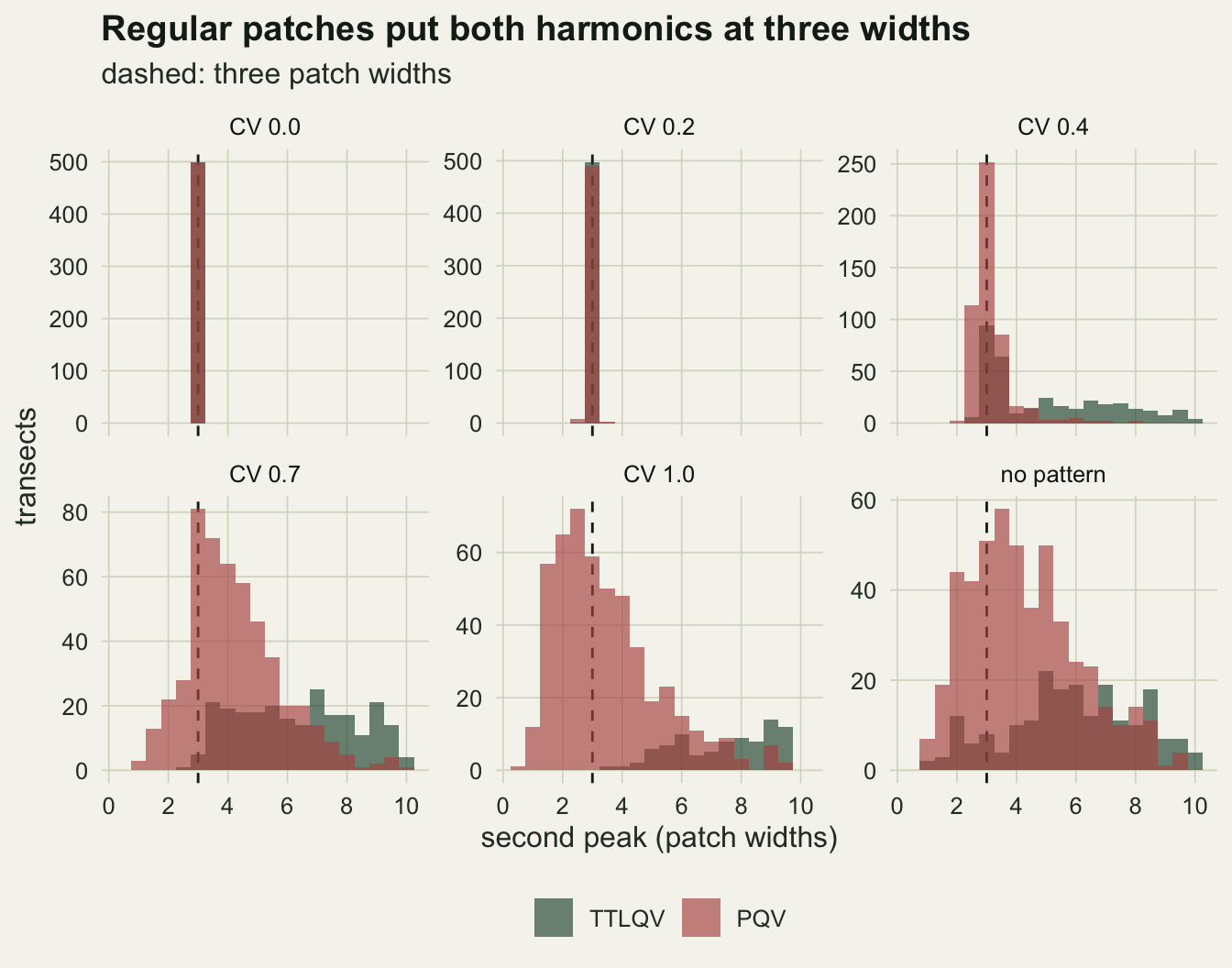
A transect that really has two scales
two_scale <- function() {
  make_transect(n_quad, w_mean, 0.4, 0) +
    make_transect(n_quad, 4 * w_mean, 0.4, 0) +
    rnorm(n_quad, 0, noise_sd)
}
set.seed(4242)
ctl <- run_condition(two_scale, "two scales")
ctl_t <- ctl[ctl$method == "TTLQV", ]
ctl_p <- ctl[ctl$method == "PQV", ]
ctl_two_t   <- mean(ctl_t$n10 >= 2)
ctl_two_p   <- mean(ctl_p$n10 >= 2)
ctl_first_t <- median(ctl_t$first, na.rm = TRUE)
ctl_small_t <- mean(!is.na(ctl_t$first) & ctl_t$first <= 1.5 * w_mean)
ctl_first_p <- median(ctl_p$first, na.rm = TRUE)
ctl_second_p <- median(ctl_p$second, na.rm = TRUE)
ctl_se <- sqrt(ctl_two_t * (1 - ctl_two_t) / n_rep)

set.seed(4243)
n_mean_curve <- 200
mean_mat <- replicate(n_mean_curve, {
  x <- two_scale()
  c(ttlqv(x, b_max), pqv(x, b_max))
})
mean_t <- rowMeans(mean_mat[1:b_max, ])
mean_p <- rowMeans(mean_mat[b_max + 1:b_max, ])
mean_peak_t <- which.max(mean_t)
mean_peak_p <- which.max(mean_p)
A positive control is needed before anything is said about what a second peak means. The transect below is the sum of two independent patterns of equal amplitude, one with mean patch and gap width 10 and one with 40, both with a CV of 0.4, plus the same noise. Four widths was chosen so that the larger scale does not fall on an odd multiple of the smaller one.
TTLQV shows two or more peaks in only 5.2 per cent of the 500 transects (standard error 0.010). Its first peak has a median of 37 quadrats, and it falls within one and a half small patch widths in 2.4 per cent of transects. The small scale is present in the data but not as a peak: TTLQV of a coarser pattern grows with block size, and the averaged curve rises through the small scale to a single maximum at 37 quadrats. PQV has a first peak with a median of 11 and a second with a median of 30, near three small widths rather than at the large width; the averaged PQV curve has its highest point at 34 quadrats, short of 40, where the rise towards the large scale meets the harmonic of the small one.
So the peak count fails in both directions on these transects: one scale gives two peaks, and two scales give one TTLQV peak and a misplaced second PQV peak.
ctl_df <- data.frame(b = rep(seq_len(b_max), 2),
                     value = c(mean_t, mean_p),
                     method = factor(rep(c("TTLQV", "PQV"), each = b_max),
                                     levels = c("TTLQV", "PQV")))
ggplot(ctl_df, aes(b, value)) +
  geom_vline(xintercept = c(w_mean, 4 * w_mean), linetype = "dashed",
             colour = te_rust, linewidth = 0.6) +
  geom_line(colour = te_forest, linewidth = 0.9) +
  facet_wrap(~ method, ncol = 2, scales = "free_y") +
  labs(x = "block size or lag (quadrats)", y = "mean variance",
       title = "Two real scales, one TTLQV peak",
       subtitle = "dashed red: the two simulated patch widths") +
  theme_datasheet()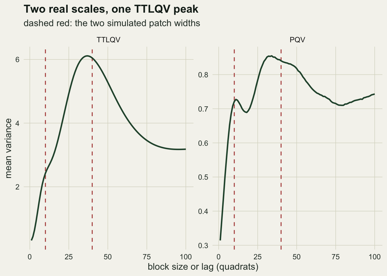
What to report
State the peak rule in the methods, with its window and its margin, and say it was fixed before the curve was examined. The replicate runs show that the number of peaks on a single-scale transect depends on the margin as much as on the pattern: at a CV of 0.4 the TTLQV rate of two or more peaks runs from 88.6 per cent at a margin of one twentieth to 30.2 per cent at one fifth. A peak list without its rule cannot be compared with anyone else’s.
Report every peak together with its ratio to the first one, both in position and in height. A second TTLQV peak near three times the first and well below half its height is the expected shape of one scale of pattern, and a reader should be told that before being told of two scales. If both TTLQV and PQV put the second peak in the same place, say so, but do not treat that agreement as confirmation: on the near-regular transects here the two methods agreed in every paired case, and there was only one scale.
Give a null alongside the curves, and say which kind. Shuffling quadrats tests for pattern of any sort; it passes the harmonic because the harmonic is pattern. A second scale needs a comparison model that has one scale and the same patch width distribution, simulated and run through the same peak rule, which is what the replicates above are. Where field cover separates cleanly into patch and gap, the observed widths can be resampled to build that model.
Show the curve to block sizes well beyond the claimed scales, and say where it was cut. The control transects show the opposite failure: TTLQV absorbed a real small scale into the rising limb of a larger one, so the absence of a peak is not the absence of a scale either.
Honest limits
The patterns are binary cover with Gaussian noise, and patch and gap widths share one gamma distribution. Real cover is graded, patches and gaps usually differ in size, and widths along a slope are rarely independent of each other. Unequal patch and gap sizes were not simulated, and the positions quoted here in patch widths should not be assumed to hold for them.
Only two of the blocked quadrat variance family were run. Three-term local quadrat variance, which compares a central block with the two either side, and the wavelet forms into which Dale and Mah recast the block methods, where other wavelet shapes are available, were not measured, and none of the rates above should be carried over to them. Dale’s book treats the whole family, and anyone choosing among the methods should start there.
The peak rule is one reasonable rule written for this post, not a rule taken from the sources cited here. A smoother rule, or one that demands a peak exceed a simulated one-scale envelope over a range of block sizes, would change every rate in the replicate table. The margins were varied to show that sensitivity, not to find a best value. One relative margin is also not the same stringency for both methods: at block size 50 the spread of the shuffled curves is 0.267 of their mean for TTLQV and 0.032 for PQV, so a margin of one tenth is 3.1 null standard deviations on PQV and 0.4 on TTLQV; in those units the rule is stricter on PQV, and PQV still finds more peaks in noise. A rule scaled to the null spread at each block size would give different rates again.
The shuffled envelope came from a single transect and was reused for all conditions after scaling by the transect variance. That is close for these binary-plus-noise transects, whose marginal distributions are similar, but it is an approximation, and a field analysis should shuffle its own data.
The positive control is one design: equal amplitudes and a four-to-one ratio of widths. A small-scale pattern with much greater amplitude than the large one might well show a TTLQV peak at its own scale, and at other width ratios the harmonics of the small scale can fall on or near the large scale and merge with it. The control shows that the failure happens, not how often across the designs a field worker might meet.
Block sizes stop at one tenth of the transect. The formulas run further, and for TTLQV the variance of the curve grows with block size, so peaks at block sizes near the end of the range were already the least reliable part of each curve.
References
Hill MO 1973 Journal of Ecology 61(1):225-235 (10.2307/2258930)
Ludwig JA, Goodall DW 1978 Vegetatio 38(1):49-59 (10.1007/BF00141298)
Guo Q, Kelly M 2004 Journal of Vegetation Science 15(6):763-770 (10.1111/j.1654-1103.2004.tb02319.x)
Dale MRT, Mah M 1998 Journal of Vegetation Science 9(6):805-814 (10.2307/3237046)
Dale MRT 1999 Spatial Pattern Analysis in Plant Ecology (ISBN 978-0-521-45227-4)