---
title: "Bayesian occupancy with latent-state MCMC"
description: "Fitting a single-season occupancy model from scratch in base R with a Gibbs sampler and data augmentation, so imperfect detection stops hiding where a species lives."
date: "2026-07-15 12:00"
categories: [R, Bayesian statistics, MCMC, occupancy, ecology tutorial]
image: thumbnail.png
image-alt: "Posterior density of occupancy probability; a dashed line marks the naive detected fraction well to the left of the posterior, and another marks the true value inside it."
---
```{r}
#| label: setup
#| include: false
knitr::opts_chunk$set(message = FALSE, warning = FALSE,
fig.width = 7.5, fig.height = 5.4, dpi = 150)
library(ggplot2)
te <- list(ink="#16241d", body="#2c3a31", forest="#275139", label="#46604a",
sage="#93a87f", paper="#f5f4ee", line="#dad9ca", faint="#5d6b61",
gold="#cda23f", mown="#2f8f63", terra="#b5534e")
theme_te <- function(base_size = 13) {
theme_minimal(base_size = base_size) +
theme(plot.background = element_rect(fill = te$paper, colour = NA),
panel.background = element_rect(fill = te$paper, colour = NA),
panel.grid.major = element_line(colour = te$line, linewidth = 0.3),
panel.grid.minor = element_blank(),
axis.text = element_text(colour = te$faint),
axis.title = element_text(colour = te$body),
plot.title = element_text(colour = te$ink, face = "bold"),
plot.subtitle = element_text(colour = te$label),
legend.text = element_text(colour = te$body),
plot.caption = element_text(colour = te$faint, size = base_size * 0.75))
}
```
A species that goes unrecorded at a site has not necessarily gone. It may have been
there and simply missed, and unless detection is perfect, the fraction of sites
where a species was seen is an undercount of the fraction where it lives. The
occupancy model separates the two probabilities, occupancy and detection, by using
repeat visits to the same sites (MacKenzie 2002). The
[frequentist version](../single-season-occupancy-model/) maximises the likelihood;
here we build the Bayesian version from scratch in base R, with a Gibbs sampler
that treats the unknown occupancy state of each undetected site as a quantity to be
sampled. That trick, sampling the missing states alongside the parameters, is data
augmentation (Tanner and Wong 1987), and it makes the whole model conditionally
conjugate.
## Simulated survey data
We survey `r 200` sites, each visited `r 4` times, for a species that occupies
`r "60%"` of sites and is detected on `r "30%"` of visits to an occupied site.
```{r}
#| label: sim
set.seed(2)
n <- 200; K <- 4; psi <- 0.6; p <- 0.3
z_t <- rbinom(n, 1, psi)                                   # true latent occupancy
Y   <- matrix(rbinom(n * K, 1, rep(z_t, K) * p), n, K)     # detection histories
det <- rowSums(Y); detected <- det > 0
naive <- mean(detected)                                    # naive detected fraction
c(detected_sites = sum(detected), all_zero = sum(!detected), naive = round(naive, 3))
```
The species was detected at `r sum(detected > 0)` of the `r n` sites, giving a
naive occupancy of `r sprintf("%.3f", naive)`, comfortably below the true
`r sprintf("%.1f", psi)`. The `r sum(!detected)` all-zero sites are the problem:
some are truly empty, and some hold the species but never showed it.
## The model and its Gibbs sampler
The model has two layers. Occupancy is `z_i ~ Bernoulli(psi)`, and detection given
occupancy is `y_ij ~ Bernoulli(z_i p)`, so a site that is empty (`z_i = 0`) can
never yield a detection. With independent `Beta(1, 1)` priors on `psi` and `p`,
every full conditional is a standard draw. A site with at least one detection must
be occupied, so its `z_i` is fixed at one. For an all-zero site, the probability
that it is occupied but undetected is the ratio below, and its `z_i` is a coin flip
with that probability. Given all the `z_i`, occupancy and detection are simple
Beta updates.
```{r}
#| label: gibbs
gibbs_occ <- function(iter = 15000, warm = 3000, seed = 1) {
  set.seed(seed)
  z <- as.integer(detected)                               # detected => occupied
  psi_s <- 0.5; p_s <- 0.5; q0 <- which(!detected)
  keep <- matrix(NA_real_, iter, 2, dimnames = list(NULL, c("psi", "p")))
  for (t in seq_len(iter)) {
    # occupied-but-undetected probability for all-zero sites, then sample z
    r <- psi_s * (1 - p_s)^K / (psi_s * (1 - p_s)^K + (1 - psi_s))
    z[q0] <- rbinom(length(q0), 1, r)
    sz <- sum(z)
    # psi | z  and  p | z, Y   are conjugate Beta draws
    psi_s <- rbeta(1, 1 + sz, 1 + n - sz)
    tot_det <- sum(det[z == 1]); tot_trials <- K * sz
    p_s <- rbeta(1, 1 + tot_det, 1 + tot_trials - tot_det)
    keep[t, ] <- c(psi_s, p_s)
  }
  keep[(warm + 1):iter, ]
}
post <- gibbs_occ(seed = 5)
psi_ci <- quantile(post[, "psi"], c(.025, .975))
p_ci   <- quantile(post[, "p"],   c(.025, .975))
round(c(psi_med = median(post[, "psi"]), psi_lo = psi_ci[1], psi_hi = psi_ci[2],
        p_med = median(post[, "p"]), p_lo = p_ci[1], p_hi = p_ci[2]), 3)
```
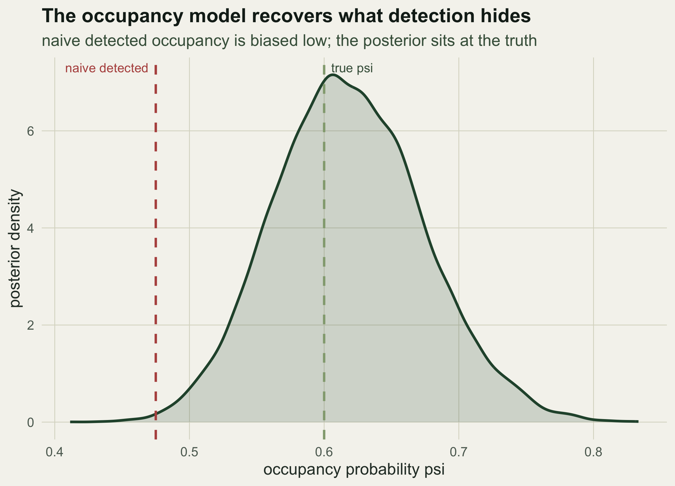
The posterior median occupancy is `r sprintf("%.3f", median(post[, "psi"]))` with a
95% credible interval of
`r sprintf("[%.3f, %.3f]", psi_ci[1], psi_ci[2])`, which brackets the true
`r sprintf("%.1f", psi)` and, more tellingly, sits entirely above the naive
`r sprintf("%.3f", naive)`: the model formally rules out the detected fraction as
too low. Detection is recovered at the same time, with a posterior median of
`r sprintf("%.3f", median(post[, "p"]))` against the true
`r sprintf("%.1f", p)`.
```{r}
#| label: fig-psi
#| fig-cap: "Posterior of occupancy probability from the Gibbs sampler. The naive detected fraction (dashed, left) falls below the whole posterior, while the true value (dashed, right) sits inside it. The model reads through the missed detections to the occupancy the raw counts understate."
#| fig-alt: "A single posterior density curve for occupancy probability, peaking near 0.62. A red dashed vertical line at about 0.48 sits to the left of the curve, and a green dashed line at 0.60 sits under the curve."
ggplot(data.frame(psi = post[, "psi"]), aes(psi)) +
  geom_density(fill = te$forest, colour = te$forest, alpha = 0.18, linewidth = 1) +
  geom_vline(xintercept = naive, colour = te$terra, linetype = "dashed", linewidth = 0.9) +
  geom_vline(xintercept = psi, colour = te$sage, linetype = "dashed", linewidth = 0.9) +
  annotate("text", x = naive, y = Inf, label = "naive detected  ", hjust = 1, vjust = 1.6,
           colour = te$terra, size = 3.6) +
  annotate("text", x = psi, y = Inf, label = "  true psi", hjust = 0, vjust = 1.6,
           colour = te$label, size = 3.6) +
  labs(x = "occupancy probability psi", y = "posterior density",
       title = "The occupancy model recovers what detection hides",
       subtitle = "naive detected occupancy is biased low; the posterior sits at the truth") +
  theme_te()
```
## Does the model fit?
A quick posterior-predictive check confirms the model reproduces the feature that
matters, the pile of all-zero sites. For each posterior draw we simulate a fresh
survey and count the sites with no detection.
```{r}
#| label: ppc
set.seed(99)
ppc_zero <- sapply(sample(nrow(post), 2000), function(i) {
  zz <- rbinom(n, 1, post[i, "psi"])
  sum(rowSums(matrix(rbinom(n * K, 1, rep(zz, K) * post[i, "p"]), n, K)) == 0)
})
c(observed = sum(!detected), predicted_median = median(ppc_zero),
  lo = quantile(ppc_zero, .05, names = FALSE), hi = quantile(ppc_zero, .95, names = FALSE))
```
The `r sum(!detected)` all-zero sites in the data sit right at the predicted median
of `r median(ppc_zero)` (90% range `r quantile(ppc_zero, .05, names = FALSE)` to
`r quantile(ppc_zero, .95, names = FALSE)`), so the mixture of truly empty and
occupied-but-missed sites is doing its job.
## What effort buys
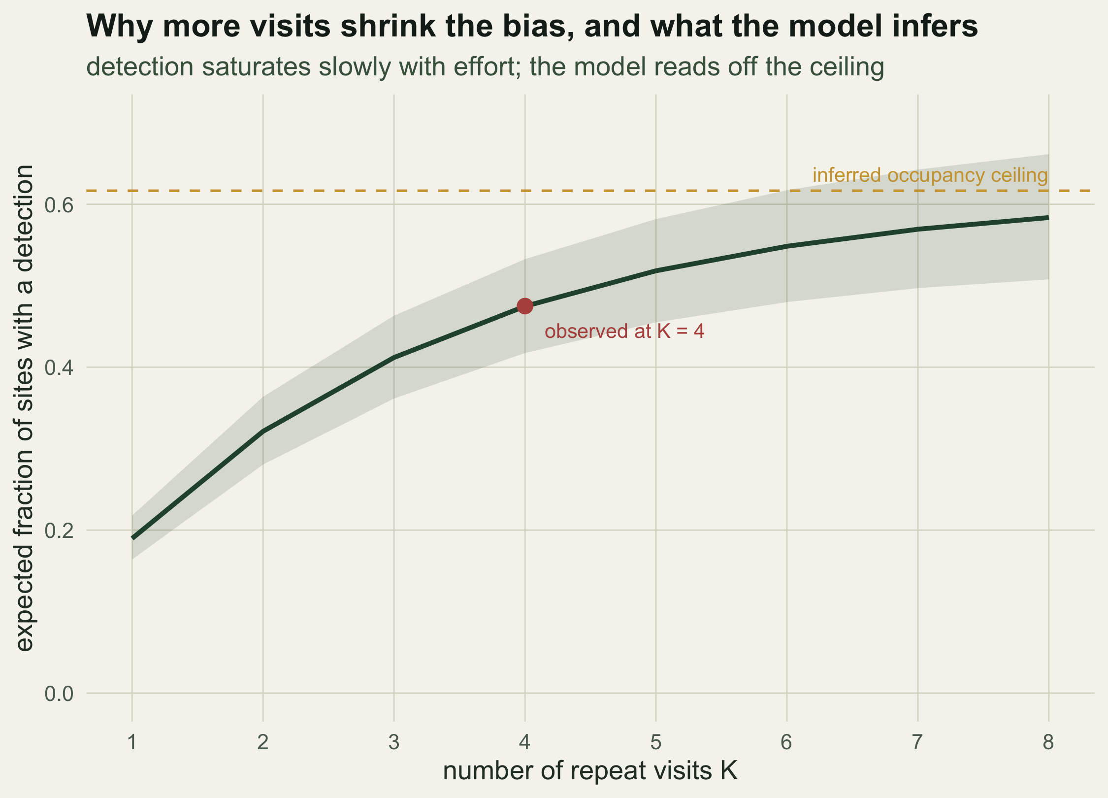
The naive undercount is not fixed, it depends on how hard you looked. The expected
fraction of sites with at least one detection is `psi (1 - (1 - p)^K)`, which
climbs towards the true occupancy as the number of visits grows. Feeding the
posterior draws through that expression traces where more effort would take the
detected fraction, and where it levels off.
```{r}
#| label: fig-effort
#| fig-cap: "Expected fraction of sites with a detection as a function of the number of repeat visits, from the posterior (band is the 90% interval). The observed detected fraction at four visits (point) lies on the curve; the curve rises towards the inferred occupancy ceiling (dashed), which four visits alone never reach."
#| fig-alt: "A rising curve of expected detected fraction against number of visits from one to eight, with a shaded band. A red point at four visits sits on the curve near 0.48. A horizontal dashed gold line near 0.62 marks the occupancy ceiling the curve approaches."
Kseq <- 1:8
band <- sapply(Kseq, function(k) quantile(post[, "psi"] * (1 - (1 - post[, "p"])^k),
                                          c(.05, .5, .95)))
dfk <- data.frame(K = Kseq, lo = band["5%", ], med = band["50%", ], hi = band["95%", ])
ggplot(dfk, aes(K, med)) +
  geom_ribbon(aes(ymin = lo, ymax = hi), fill = te$forest, alpha = 0.15) +
  geom_line(colour = te$forest, linewidth = 1.1) +
  geom_hline(yintercept = median(post[, "psi"]), colour = te$gold, linetype = "dashed") +
  geom_point(data = data.frame(K = K, naive = naive), aes(K, naive),
             colour = te$terra, size = 3) +
  annotate("text", x = 8, y = median(post[, "psi"]) + 0.02, hjust = 1, colour = te$gold,
           size = 3.5, label = "inferred occupancy ceiling") +
  annotate("text", x = K + 0.15, y = naive - 0.03, hjust = 0, colour = te$terra,
           size = 3.5, label = "observed at K = 4") +
  coord_cartesian(ylim = c(0, 0.7)) + scale_x_continuous(breaks = Kseq) +
  labs(x = "number of repeat visits K", y = "expected fraction of sites with a detection",
       title = "Why more visits shrink the bias, and what the model infers",
       subtitle = "detection saturates slowly with effort; the model reads off the ceiling") +
  theme_te()
```
## Assumptions worth stating
The model earns its correction by assuming a few things. The sites are closed over
the survey, so occupancy does not change between the first visit and the last; a
detection is never a false positive, so seeing the species means it is there; and
detection is constant across visits and sites, which is easy to relax by letting
`p` depend on covariates through a logit link, exactly as in an ordinary logistic
model. When detection is genuinely low, occupancy stays uncertain no matter how the
model is fitted, which is why the posterior here is wide rather than sharp. That
width is the honest report. The one thing that is not defensible is the naive
count, which answers a different and easier question, how often the species was
seen, and quietly lets it stand in for how often it was there.
A non-detection is not an absence. The latent-state model turns that sentence into
arithmetic: it holds a probability that each quiet site is occupied, averages over
those probabilities, and returns the occupancy rate with the uncertainty it
deserves.
## References
- MacKenzie DI, Nichols JD, Lachman GB, Droege S, Royle JA, Langtimm CA 2002 Ecology 83(8):2248-2255 (10.1890/0012-9658(2002)083[2248:ESORWD]2.0.CO;2)
- Tanner MA, Wong WH 1987 Journal of the American Statistical Association 82(398):528-540 (10.1080/01621459.1987.10478458)
- Kery M, Schaub M 2012 Bayesian Population Analysis using WinBUGS (ISBN 978-0-12-387020-9)
- Kery M, Royle JA 2016 Applied Hierarchical Modeling in Ecology, Volume 1 (ISBN 978-0-12-801378-6)
## Related tutorials
- [Single-season occupancy models](../single-season-occupancy-model/)
- [Imperfect detection and occupancy](../imperfect-detection-occupancy/)
- [Gibbs sampling with conjugate priors](../gibbs-sampling-conjugate/)
- [Bayesian hierarchical models with MCMC](../bayesian-hierarchical-model-mcmc/)