library(vegan)
library(ggplot2)

theme_te <- function(base_size = 12) {
  theme_minimal(base_size = base_size) +
    theme(
      plot.background  = element_rect(fill = "#f5f4ee", colour = NA),
      panel.background = element_rect(fill = "#f5f4ee", colour = NA),
      panel.grid.major = element_line(colour = "#dad9ca", linewidth = 0.3),
      panel.grid.minor = element_blank(),
      axis.text   = element_text(colour = "#46604a"),
      axis.title  = element_text(colour = "#2c3a31"),
      plot.title  = element_text(colour = "#16241d", face = "bold"),
      plot.subtitle = element_text(colour = "#5d6b61"),
      strip.text  = element_text(colour = "#16241d", face = "bold"),
      legend.position = "none"
    )
}
forest <- "#275139"; label <- "#46604a"; sage <- "#93a87f"
red <- "#b5534e"; faint <- "#5d6b61"Additive diversity partitioning in R
ecology tutorial
R
vegan
beta diversity
community ecology
Hill numbers
Split gamma diversity into alpha and beta additively in R with vegan adipart, test it with a null model, and see why Hill numbers matter for diversity indices.
Regional diversity is more than the diversity of any one site. Whittaker’s classic answer was multiplicative, gamma equals alpha times beta, so beta measured how many times richer a region was than an average site. Lande (1996) offered an additive alternative, gamma equals alpha plus beta, which keeps alpha and beta in the same units and lets you stack the pieces of a sampling hierarchy on top of one another. This post partitions richness additively in R with vegan, tests the result against a null model, and then shows why the additive form needs care once you move from counting species to diversity indices.
The additive identity
Additive partitioning writes total diversity as a sum:
gamma = alpha + beta
where alpha is the mean diversity of a single sample and beta is the average amount by which the whole exceeds a part. When samples are grouped into regions, the identity extends to as many levels as the design has:
gamma = mean sample alpha + (among samples within regions) + (among regions)
Every term is in species, so a beta of 20 means twenty species of turnover, full stop. That shared currency is what makes additive partitioning easy to read and easy to draw. The multiplicative form of Whittaker, and the dissimilarity-based framework of Baselga, answer related questions in different currencies, and are worth keeping separate in your head.
Partitioning richness with adipart
We simulate a two-level design: three regions, five samples each, with overlapping species pools so that neighbouring regions share some species while distant ones do not. Within a region, each sample draws a subset of the regional pool.
set.seed(20)
nreg <- 3; per <- 5; nsamp <- nreg * per; npool <- 60
region <- factor(rep(paste0("R", 1:nreg), each = per))
comm <- matrix(0, nsamp, npool)
for (k in 1:nreg) {
  start <- (k - 1) * 16 + 1
  pool  <- start:min(start + 27, npool)          # overlapping regional pool
  for (r in which(region == paste0("R", k))) {
    present <- sample(pool, size = sample(10:16, 1))
    comm[r, present] <- rpois(length(present), 4) + 1
  }
}
comm <- comm[, colSums(comm) > 0]
c(samples = nrow(comm), species = ncol(comm), gamma = sum(colSums(comm) > 0))
samples species gamma
15 58 58 adipart takes the community matrix and a grouping formula. With comm ~ region it recognises two grouping levels, the sample (each row) and the region, and returns alpha and beta at each. The weights = "unif" setting gives every unit equal weight; index = "richness" partitions species counts.
dat <- data.frame(region = region)
set.seed(5)
ap <- adipart(comm ~ region, dat, index = "richness",
              weights = "unif", nsimul = 999)
S <- ap$statistic
a1 <- S[["alpha.1"]]; b1 <- S[["beta.1"]]
a2 <- S[["alpha.2"]]; b2 <- S[["beta.2"]]; g <- S[["gamma"]]
round(c(alpha.sample = a1, beta.within = b1,
        alpha.region = a2, beta.among = b2, gamma = g), 1)
alpha.sample beta.within alpha.region beta.among gamma
13.6 13.4 27.0 31.0 58.0 The mean sample holds 13.6 species. Within a region, samples add 13.4 species of turnover, bringing the regional mean to 27. The three regions then add another 31 species, reaching the total of 58. The whole decomposition is one sum: 13.6 plus 13.4 plus 31 equals 58.
comp <- data.frame(
  part = factor(c("mean sample richness (alpha)",
                  "among samples within region (beta 1)",
                  "among regions (beta 2)"),
                levels = c("among regions (beta 2)",
                           "among samples within region (beta 1)",
                           "mean sample richness (alpha)")),
  value = c(a1, b1, b2))
comp$lab <- sprintf("%.1f", comp$value)

ggplot(comp, aes(x = "community", y = value, fill = part)) +
  geom_col(width = 0.5, colour = "#f5f4ee", linewidth = 0.6) +
  geom_text(aes(label = lab), position = position_stack(vjust = 0.5),
            colour = c("#16241d", "#16241d", "white"), size = 4.4, fontface = "bold") +
  annotate("text", x = "community", y = g + 1.2,
           label = paste0("gamma = ", sprintf("%.0f", g)),
           colour = "#16241d", fontface = "bold", size = 4.2, hjust = 0) +
  scale_fill_manual(values = c("mean sample richness (alpha)" = forest,
                               "among samples within region (beta 1)" = sage,
                               "among regions (beta 2)" = label),
                    guide = guide_legend(reverse = TRUE)) +
  scale_y_continuous(limits = c(0, 72), expand = expansion(mult = c(0, 0))) +
  coord_flip() +
  labs(x = NULL, y = "species richness",
       title = "Additive partition: gamma = alpha + beta, in species",
       subtitle = "total richness splits into mean local richness plus two turnover layers") +
  theme_te() +
  theme(legend.position = "top", legend.title = element_blank(),
        legend.text = element_text(colour = "#2c3a31", size = 8.5),
        axis.text.y = element_blank())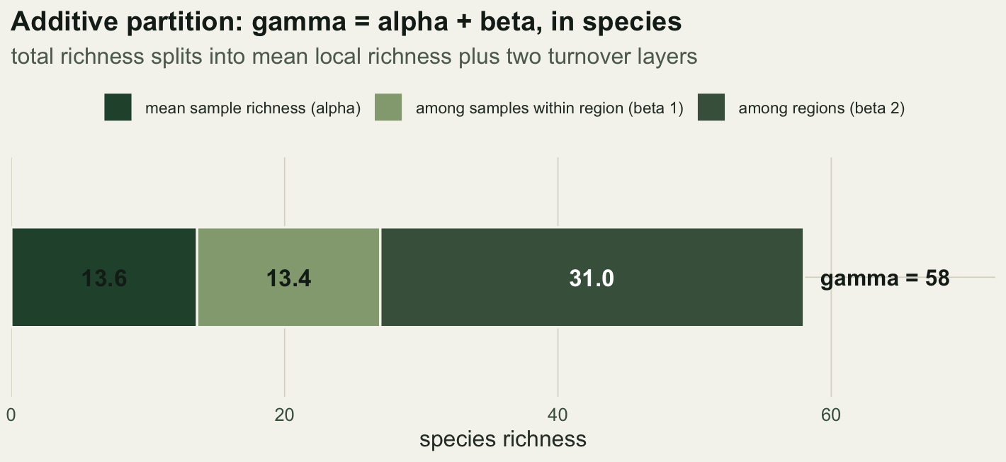
Testing against a null model
The numbers describe the data, but are they more structured than chance? adipart answers this with a randomisation test built on the r2dtable null model, which reshuffles individuals across the whole table while holding the row and column totals fixed. This individual-based null (Crist and colleagues 2003) asks what the partition would look like if individuals ignored the regional structure entirely. The observed statistics come with a z-score and a permutation p for each level.
z  <- ap$oecosimu$z;    names(z)  <- names(S)
p  <- ap$oecosimu$pval; names(p)  <- names(S)
mn <- ap$oecosimu$means; names(mn) <- names(S)
round(c(among_region_obs = b2, among_region_null = mn[["beta.2"]],
        z = z[["beta.2"]], p = p[["beta.2"]]), 2)
among_region_obs among_region_null z p
31.00 1.80 48.02 0.00 Among-region turnover is the headline. Its observed value of 31 towers over the null mean of 1.8, with a z of 48 and a permutation p of 0.001. Under the null, spreading individuals at random across all fifteen samples would leave the regions nearly identical; the real data keep them sharply distinct.
dfb <- data.frame(beta2 = ap$oecosimu$simulated[5, ])

ggplot(dfb, aes(beta2)) +
  geom_histogram(bins = 40, fill = forest, colour = NA, alpha = 0.85) +
  geom_vline(xintercept = b2, colour = red, linewidth = 0.8) +
  annotate("text", x = b2 - 1, y = Inf, label = paste0("observed = ", sprintf("%.0f", b2)),
           hjust = 1, vjust = 1.8, colour = red, size = 3.6, fontface = "bold") +
  annotate("text", x = 6, y = Inf,
           label = paste0("null mean = ", sprintf("%.1f", mn[["beta.2"]]),
                          "\nz = ", sprintf("%.0f", z[["beta.2"]])),
           hjust = 0, vjust = 1.6, colour = faint, size = 3.5) +
  scale_y_continuous(expand = expansion(mult = c(0, 0.08))) +
  labs(x = "among-region beta under the individual-based null", y = "count",
       title = "Regional turnover far exceeds chance",
       subtitle = "observed among-region beta against 999 randomised communities") +
  theme_te()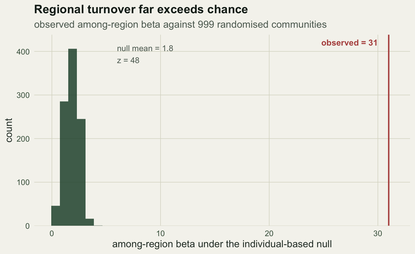
Turnover among samples within a region tells the opposite story. Its observed value of 13.4 sits below the null mean of 19.7, giving a negative z of -8.3. Samples from the same region are more alike than random reassignment would make them, which is what a shared regional pool should produce.
Additive or multiplicative?
For richness, the additive form behaves well: species are counts, and a difference of counts is again a count. Trouble appears when the same additive recipe is applied to a diversity index such as Gini-Simpson. The identity still holds arithmetically, but the beta it produces is not comparable across studies, because its size depends on how much alpha diversity there is to begin with.
A short demonstration makes the problem concrete. Hold the ecology fixed at three fully distinct regions, each with the same number of equally abundant species, and vary that number. The regions are always completely different, so any honest measure of differentiation should return the same value. Additive Gini-Simpson beta does not.
N <- 3; Sseq <- 2:30
demo <- data.frame(
  S         = Sseq,
  add_GS    = (1 - 1 / (N * Sseq)) - (1 - 1 / Sseq),   # additive Gini-Simpson
  mult_Hill = (N * Sseq) / Sseq)                       # multiplicative Hill, q = 2
c(add_GS_low = demo$add_GS[1], add_GS_high = demo$add_GS[length(Sseq)],
  mult_Hill  = demo$mult_Hill[1])
add_GS_low add_GS_high mult_Hill
0.33333333 0.02222222 3.00000000 As local richness climbs, additive Gini-Simpson beta falls from 0.333 towards 0.022, sliding towards zero even though the regions stay just as distinct. The multiplicative partition of Hill numbers avoids this. Converting Simpson to its numbers equivalent (an effective species count) and dividing gamma by alpha gives beta as an effective number of communities, which stays pinned at 3 regardless of richness. That is the value the ecology demands.
dd <- rbind(
  data.frame(S = demo$S, beta = demo$add_GS,    panel = "additive (Gini-Simpson index)"),
  data.frame(S = demo$S, beta = demo$mult_Hill, panel = "multiplicative (Hill numbers, q = 2)"))
dd$panel <- factor(dd$panel, levels = c("additive (Gini-Simpson index)",
                                        "multiplicative (Hill numbers, q = 2)"))

ggplot(dd, aes(S, beta)) +
  geom_line(colour = forest, linewidth = 1) +
  geom_point(colour = forest, size = 1.3) +
  facet_wrap(~panel, scales = "free_y") +
  labs(x = "species per region (local richness)", y = "beta diversity",
       title = "Why the choice of index matters",
       subtitle = "three fully distinct regions throughout; only the diversity index differs") +
  theme_te() +
  theme(strip.text = element_text(size = 10.5))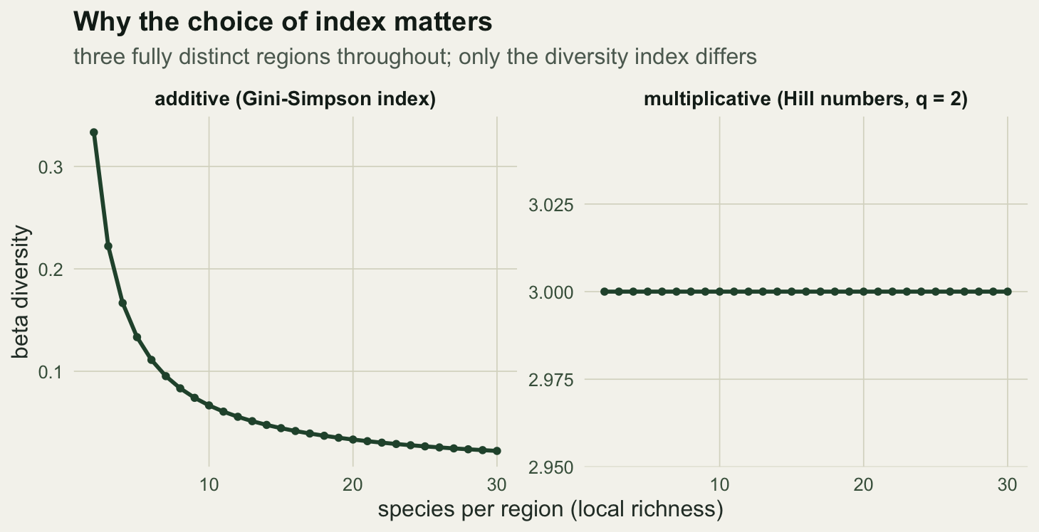
Shannon sits in between. Its entropy is additive, so the sample and turnover entropies do add to the total, but entropy is measured in nats, not communities. Exponentiating turns Shannon entropy into a Hill number, and at that point the partition becomes multiplicative again. The clean way to think about it is that raw indices partition additively while their numbers equivalents partition multiplicatively, and only the numbers equivalents give a beta you can compare across datasets.
What to take away
Additive partitioning with adipart is a direct, testable way to break total richness into local diversity and layers of turnover, and its randomisation test tells you which layers exceed chance. Read the species-based partition at face value. But the moment you partition a diversity index rather than a raw species count, convert to Hill numbers and partition multiplicatively, so that beta means a number of distinct communities that does not secretly depend on how rich your sites happen to be.
References
Lande, R. 1996. Oikos 76(1):5-13 (10.2307/3545743).
Crist, T.O., Veech, J.A., Gering, J.C. and Summerville, K.S. 2003. American Naturalist 162(6):734-743 (10.1086/378901).
Jost, L. 2007. Ecology 88(10):2427-2439 (10.1890/06-1736.1).
Veech, J.A., Summerville, K.S., Crist, T.O. and Gering, J.C. 2002. Oikos 99(1):3-9 (10.1034/j.1600-0706.2002.990101.x).