---
title: "Stage-structured Lefkovitch matrices in R"
description: "Build a stage-classified Lefkovitch matrix in R for a plant with variable stage durations, and see why the diagonal stasis term is not optional bookkeeping."
date: 2026-07-05 11:00
categories: [R, population dynamics, matrix models, stage structure, ecology tutorial]
image: thumbnail.png
image-alt: "Heatmap of a four by four stage matrix showing fecundity, stasis and growth entries"
---
For many organisms, age is the wrong currency. A small and a large plant of the same age can have completely different survival and reproduction, and a big individual that shrank one year might still be big the next. When fate depends on size or developmental stage rather than chronological age, the [Leslie matrix](../leslie-matrix-population-models/) gives way to a stage-classified matrix, introduced by Lefkovitch in 1965. This post builds one for a perennial plant, reads its growth rate and stable stage distribution with the same eigenvalue machinery, and shows why the one structural difference from a Leslie matrix, a non-zero diagonal, carries most of the survival.
## Stages instead of ages
The difference is entirely in the matrix structure. A Leslie matrix forces every individual to advance one age class per year, so its diagonal is zero. A stage matrix lets individuals stay in the same stage from one year to the next, because a stage can last a variable number of years. That staying probability sits on the diagonal and is called stasis.
```{r}
#| label: setup
#| message: false
#| warning: false
library(ggplot2)
library(dplyr)
library(tidyr)

te_ink <- "#16241d"; te_forest <- "#275139"; te_mown <- "#2f8f63"
te_gold <- "#c9b458"; te_faint <- "#5d6b61"; te_line <- "#dad9ca"; te_paper <- "#f5f4ee"
theme_te <- function(base_size = 12) {
  theme_minimal(base_size = base_size) +
    theme(text = element_text(colour = "#2c3a31"),
          plot.title = element_text(colour = te_ink, face = "bold", size = base_size * 1.15),
          plot.subtitle = element_text(colour = te_faint, size = base_size * 0.95),
          axis.title = element_text(colour = "#46604a"), axis.text = element_text(colour = te_faint),
          panel.grid.minor = element_blank(),
          panel.grid.major = element_line(colour = te_line, linewidth = 0.3),
          plot.background = element_rect(fill = te_paper, colour = NA),
          panel.background = element_rect(fill = te_paper, colour = NA),
          legend.key = element_rect(fill = te_paper, colour = NA))
}

stages <- c("Seedling", "Juvenile", "Small adult", "Large adult")
A <- matrix(0, 4, 4, dimnames = list(stages, stages))
A["Juvenile",    "Seedling"]    <- 0.30   # survive and grow
A["Juvenile",    "Juvenile"]    <- 0.35   # stasis
A["Small adult", "Juvenile"]    <- 0.30   # survive and grow
A["Small adult", "Small adult"] <- 0.45   # stasis
A["Large adult", "Small adult"] <- 0.25   # survive and grow
A["Seedling",    "Small adult"] <- 1.60   # fecundity
A["Large adult", "Large adult"] <- 0.82   # stasis
A["Seedling",    "Large adult"] <- 3.00   # fecundity
A
```
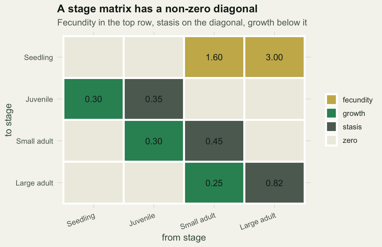
Read the matrix by columns: each column says where an individual currently in that stage goes next year. A small adult (column three) stays small with probability 0.45, grows to large with probability 0.25, and produces on average 1.60 seedlings. Total survival for a small adult is 0.45 plus 0.25, which is 0.70. The two entries in the top row are fecundities; everything on and below the diagonal is survival.
```{r}
#| label: fig-structure
#| fig-cap: "The stage matrix: fecundity in the top row, stasis on the diagonal, growth below."
#| fig-alt: "A four by four grid of matrix entries coloured by role: two gold fecundity cells in the top row, grey stasis cells on the diagonal, green growth cells just below the diagonal, and pale zeros elsewhere."
#| fig-width: 6.8
#| fig-height: 4.4
df <- as.data.frame(as.table(A))
colnames(df) <- c("to", "from", "value")
df$to   <- factor(df$to,   levels = rev(stages))
df$from <- factor(df$from, levels = stages)
df$kind <- "zero"
df$kind[df$value > 0 & as.character(df$to) == "Seedling"] <- "fecundity"
df$kind[df$value > 0 & as.character(df$from) == as.character(df$to)] <- "stasis"
df$kind[df$value > 0 & df$kind == "zero"] <- "growth"
df$lab <- ifelse(df$value > 0, sprintf("%.2f", df$value), "")
ggplot(df, aes(from, to, fill = kind)) +
  geom_tile(colour = "white", linewidth = 1.2) +
  geom_text(aes(label = lab), colour = te_ink, size = 4) +
  scale_fill_manual(values = c(zero = "#eeece1", fecundity = te_gold,
                               stasis = te_faint, growth = te_mown), name = NULL) +
  labs(title = "A stage matrix has a non-zero diagonal",
       subtitle = "Fecundity in the top row, stasis on the diagonal, growth below it",
       x = "from stage", y = "to stage") +
  theme_te() +
  theme(panel.grid = element_blank(), axis.text.x = element_text(angle = 20, hjust = 1))
```
## The same eigenvalue analysis
Nothing about the analysis changes. The dominant eigenvalue is still the asymptotic growth rate, and the right eigenvector is still the stable distribution, now over stages rather than ages.
```{r}
#| label: eigen
ev  <- eigen(A)
lam <- Re(ev$values[1])
w   <- Re(ev$vectors[, 1]); w <- w / sum(w)
c(lambda = lam)
round(100 * w, 1)
```
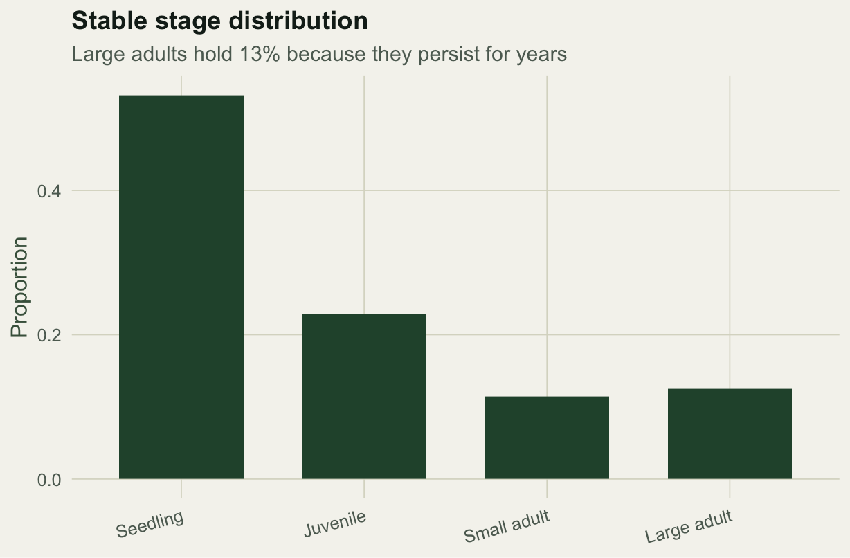
The population grows about five percent a year. At the stable structure just over half the individuals are seedlings, a signature of high seed output paired with low seedling survival. Notice that large adults hold a slightly larger share than small adults even though fewer individuals reach them, because they persist for years once there.
```{r}
#| label: fig-stable
#| fig-cap: "Stable stage distribution; the long-lived large-adult stage accumulates individuals."
#| fig-alt: "Bar chart of the stable stage distribution across four stages, dominated by seedlings at over fifty percent and falling to about twelve percent for large adults."
#| fig-width: 6.4
#| fig-height: 4.2
data.frame(stage = factor(stages, levels = stages), w = w) |>
  ggplot(aes(stage, w)) +
  geom_col(fill = te_forest, width = 0.68) +
  labs(title = "Stable stage distribution",
       subtitle = sprintf("Large adults hold %.0f%% because they persist for years", 100 * w[4]),
       x = NULL, y = "Proportion") +
  theme_te() + theme(axis.text.x = element_text(angle = 15, hjust = 1))
```
## How long individuals linger
The diagonal has a direct reading. If the probability of staying in a stage is `s`, then the expected number of years an individual spends there before leaving, whether by growing on or dying, follows a geometric distribution with mean `1 / (1 - s)`.
```{r}
#| label: residence
stasis    <- diag(A)
residence <- 1 / (1 - stasis)
round(residence, 2)
```
Seedlings spend a single year in their stage, since they either become juveniles or die within the year. Large adults linger for more than five years on average. That long residence is exactly what a chronological-age model cannot capture without an unwieldy number of age classes.
## Stasis is not optional
It is tempting to think of the diagonal as a modelling convenience. It is not. For a long-lived stage, most of the survival lives on the diagonal. Zeroing it out, which is what treating the model as an age-structured Leslie matrix would force, removes that survival and collapses the population.
```{r}
#| label: no-stasis
A_nostasis <- A
diag(A_nostasis) <- 0
lam_nostasis <- Re(eigen(A_nostasis)$values[1])
c(with_stasis = lam, without_stasis = lam_nostasis)
```
Deleting stasis turns a population growing at 1.05 into one crashing at 0.63, because large adults, stripped of their staying-alive-in-place survival, now vanish every year. The lesson is that stage duration is a real biological quantity, and the diagonal is where it lives.
## What to take away
A stage-classified Lefkovitch matrix is the right tool when size or developmental stage, not age, determines an individual's fate. Structurally it differs from a Leslie matrix in one place, the diagonal, which holds the probability of staying in a stage and encodes variable stage durations. The eigenvalue analysis is identical: dominant eigenvalue for growth rate, right eigenvector for the stable stage distribution. For where to find real stage matrices across a thousand plant species, the COMPADRE database is the standard source. The question of which matrix entries most affect growth, and whether protecting stasis or fecundity buys more, is the subject of sensitivity and elasticity analysis.
## References
- Lefkovitch LP 1965 Biometrics 21(1):1-18 (10.2307/2528348)
- Werner PA, Caswell H 1977 Ecology 58:1103-1111 (pre-DOI)
- Caswell H 2001 Matrix Population Models, 2nd ed, Sinauer Associates (ISBN 978-0-87893-096-8)
- Salguero-Gomez R et al 2015 Journal of Ecology 103(1):202-218 (10.1111/1365-2745.12334)
- Gotelli NJ 2008 A Primer of Ecology, 4th ed, Sinauer Associates (ISBN 978-0-87893-318-1)
## Related tutorials
- [Leslie matrix population models in R](../leslie-matrix-population-models/)
- [Sensitivity and elasticity of matrix models](../matrix-sensitivity-elasticity/)
- [Life tables and population growth in R](../life-tables-and-lambda/)