library(spdep)

set.seed(54)
n <- 150
coords <- cbind(x = runif(n, 0, 10), y = runif(n, 0, 10))
Dm <- as.matrix(dist(coords))

rfield <- function(D, range, sd = 1){            # Gaussian field, exponential covariance
  Sigma <- sd^2 * exp(-D / range)
  L <- chol(Sigma + diag(1e-9, nrow(D)))
  as.vector(crossprod(L, rnorm(nrow(D))))
}
env   <- rfield(Dm, range = 2.5)                        # measured predictor, spatially structured
sp2   <- residuals(lm(rfield(Dm, range = 2.0) ~ env))   # a second driver, made orthogonal to env
y     <- 1.0 + 1.5 * env + 1.2 * sp2 + rnorm(n, 0, 0.6) # response we model further down
randv <- rnorm(n) # a variable with no spatial structureSpatial autocorrelation and Moran’s I: when sites are not independent
R
spatial
spdep
regression
Nearby sites tend to resemble each other, which breaks the independence that regression assumes. Moran’s I measures it, a correlogram shows its scale, and a residual test catches it before it inflates your false positives.
The regression posts on this blog, the count GLM and the GAM, all rest on one quiet assumption: the observations are independent. For data collected across space, that assumption is usually wrong. Sites near each other tend to have similar values, whether because the environment varies smoothly or because of processes like dispersal and local interaction. This is spatial autocorrelation, and it violates the independence that standard tests need (Legendre 1993). When it goes unnoticed it does real damage: it shrinks the effective sample size, deflates standard errors, and can turn noise into a significant result.
This post measures spatial autocorrelation with Moran’s I using spdep, shows how it changes with distance through a correlogram, uses it as a diagnostic on regression residuals, and then demonstrates what it does to a test that ignores it.
A spatially structured variable
The sampling points are scattered over a square. The environmental variable is a Gaussian random field with an exponential covariance, so nearby points are correlated and the correlation fades with distance. The same block also defines a second spatial driver and a response built from both, which we return to for the regression diagnostic.
ggplot(data.frame(coords, env), aes(x, y, color = env)) +
  geom_point(size = 2.6) +
  scale_color_gradient(low = pal$low, high = pal$high, name = "env") +
  coord_equal() + labs(x = "Easting", y = "Northing") + th()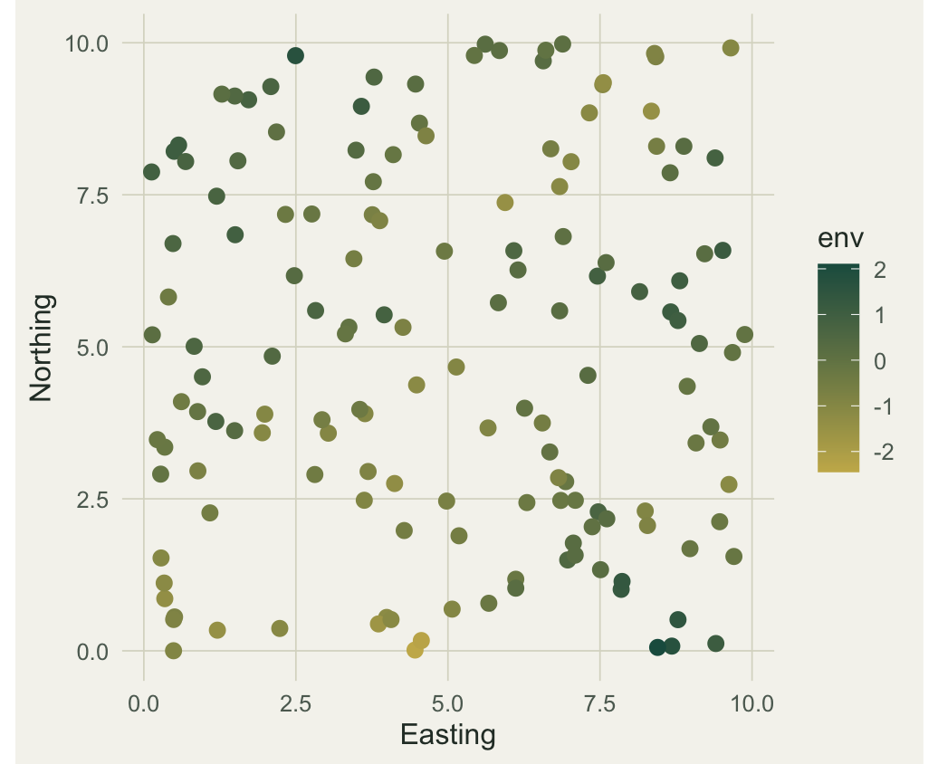
Moran’s I
Moran’s I is a correlation coefficient for a variable with itself across space. Each pair of sites contributes the product of their two deviations from the mean, weighted by how much the two sites count as neighbours. If neighbouring sites tend to be on the same side of the mean, I is positive (clustering); if they alternate, I is negative (a checkerboard). Under no spatial pattern the expected value is not zero but slightly below it, at minus one over (n minus one).
The weights come from a neighbour definition. Here every site is linked to its eight nearest neighbours, and the links are row-standardized so each site’s neighbours sum to one.
nb <- knn2nb(knearneigh(coords, k = 8))
lw <- nb2listw(nb, style = "W")
-1 / (n - 1)            # expected I under no autocorrelation
[1] -0.006711409A permutation test compares the observed I to its distribution under random reshuffling of the values across locations. Run it on the structured variable and on a variable with no spatial pattern.
set.seed(1); mi_env  <- moran.mc(env, lw, nsim = 999)
set.seed(1); mi_rand <- moran.mc(randv, lw, nsim = 999)
c(env_I = round(mi_env$statistic, 3),    env_p = mi_env$p.value,
  random_I = round(mi_rand$statistic, 3), random_p = mi_rand$p.value)
env_I.statistic env_p random_I.statistic random_p
0.523 0.001 -0.061 0.933 The structured variable has an I near 0.52, far above its expectation and significant at the permutation floor. The random variable sits close to zero, indistinguishable from its expected value, and is not significant. Moran’s I is doing what it should: flagging the spatial pattern and ignoring its absence.
How far does it reach?
A single Moran’s I summarizes autocorrelation at the scale of the neighbour definition. A correlogram breaks it out by distance: compute I using only pairs of sites within each distance band, and watch it decay.
breaks <- seq(0, 8, by = 1)
corr <- data.frame(lo = head(breaks, -1), hi = tail(breaks, -1), I = NA, p = NA)
for (i in seq_len(nrow(corr))){
  nbd <- dnearneigh(coords, corr$lo[i], corr$hi[i])
  if (sum(card(nbd)) > 0){
    lwd <- nb2listw(nbd, style = "W", zero.policy = TRUE)
    mm  <- moran.test(env, lwd, zero.policy = TRUE)
    corr$I[i] <- mm$estimate[1]; corr$p[i] <- mm$p.value
  }
}
corr$mid <- (corr$lo + corr$hi) / 2
corr$sig <- ifelse(corr$p < 0.05, "p < 0.05", "ns")

ggplot(corr, aes(mid, I)) +
  geom_hline(yintercept = -1/(n-1), linetype = "22", color = pal$faint) +
  geom_line(color = pal$sage, linewidth = .6) +
  geom_point(aes(color = sig), size = 3) +
  scale_color_manual(values = c("p < 0.05" = pal$forest, "ns" = pal$gold), name = NULL) +
  labs(x = "Distance class (midpoint)", y = "Moran's I") + th() +
  theme(legend.position = "top")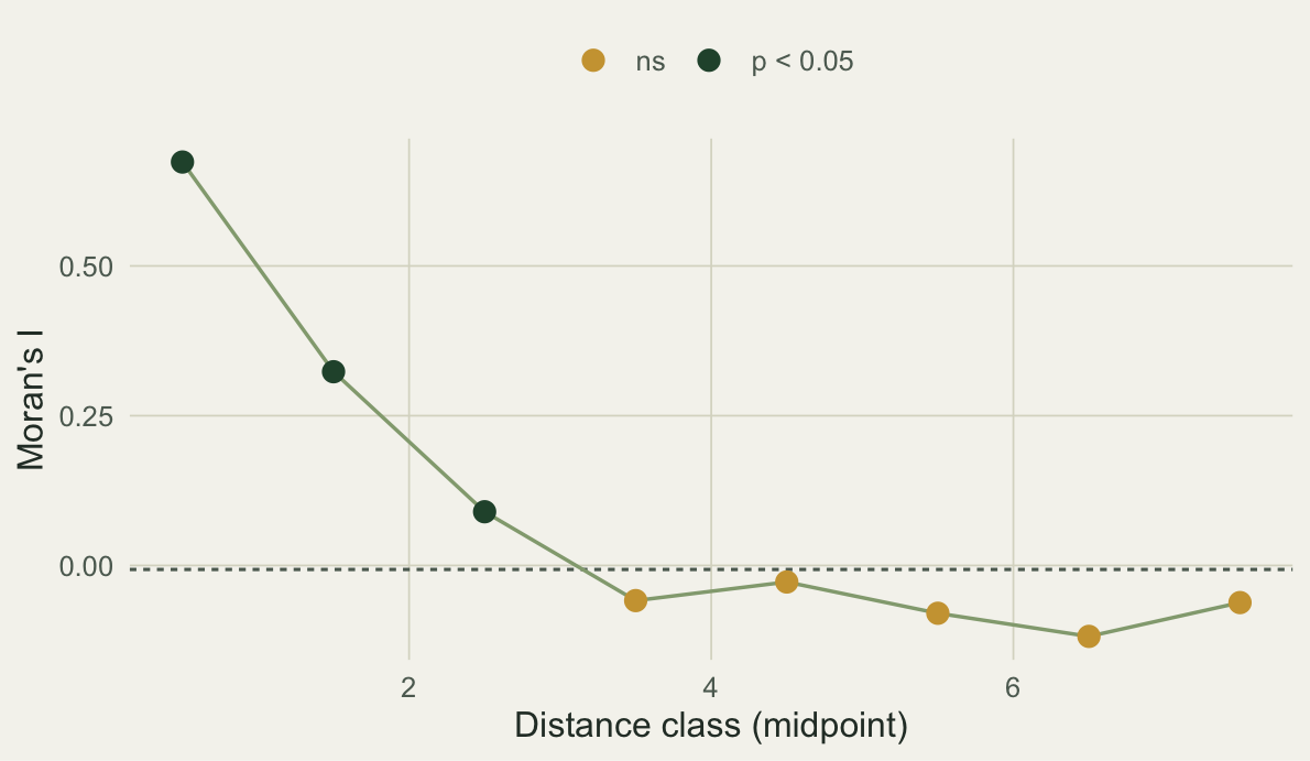
Autocorrelation is around 0.67 for the closest pairs, halves by the next band, and has faded into non-significance past a distance of about three, which is close to the field’s range of 2.5. Sites farther apart than that carry no detectable spatial dependence.
The regression diagnostic
Here is where Moran’s I earns its place in a modeling workflow. The response y defined earlier depends on env plus a second spatial driver sp2, which we now treat as unmeasured. Fit the obvious model that uses only env, then look at its residuals.
m1 <- lm(y ~ env)            # omits the second driver
m2 <- lm(y ~ env + sp2)      # includes it

set.seed(1); r1 <- moran.mc(residuals(m1), lw, nsim = 999)
set.seed(1); r2 <- moran.mc(residuals(m2), lw, nsim = 999)
rbind(
  `y ~ env`        = c(env_coef = coef(m1)[2], resid_I = r1$statistic, p = r1$p.value),
  `y ~ env + sp2`  = c(env_coef = coef(m2)[2], resid_I = r2$statistic, p = r2$p.value))
env_coef.env resid_I.statistic p
y ~ env 1.583541 0.467886475 0.001
y ~ env + sp2 1.583541 0.001633636 0.387Both models put the same coefficient on env, near the true value of 1.5. The difference is in the residuals. The first model leaves out the second spatial driver, so its residuals still carry that structure: Moran’s I near 0.47, strongly significant. The second model captures it, and its residuals are spatially flat, with an I indistinguishable from zero. The point estimate looked fine either way; only the residual test revealed that the first model’s assumptions were broken.
rd <- rbind(
  data.frame(coords, resid = residuals(m1),
             model = sprintf("y ~ env  (residual I = %.2f)", r1$statistic)),
  data.frame(coords, resid = residuals(m2),
             model = sprintf("y ~ env + sp2  (residual I = %.2f)", r2$statistic)))
lim <- max(abs(rd$resid))
ggplot(rd, aes(x, y, color = resid)) +
  geom_point(size = 2.2) + facet_wrap(~model) +
  scale_color_gradient2(low = pal$terra, mid = pal$paper, high = pal$high,
                        midpoint = 0, limits = c(-lim, lim), name = "resid") +
  coord_equal() + labs(x = "Easting", y = "Northing") + th()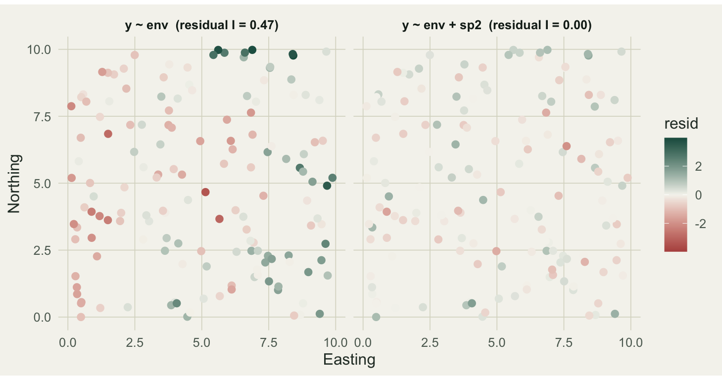
Why a flat residual map matters
Leaving autocorrelation in the residuals is not a cosmetic problem. The standard errors and p values from lm assume independent residuals; when the residuals are autocorrelated, those numbers are not trustworthy, and with positive autocorrelation they are usually too optimistic. The cleanest way to see the cost is a simulation: regress one spatial field on a second, unrelated spatial field, where the true slope is zero, and count how often the test calls it significant.
type1 <- function(nrep, n, range, alpha = 0.05){
  rej_sp <- 0; rej_iid <- 0
  for (r in 1:nrep){
    co <- cbind(runif(n, 0, 10), runif(n, 0, 10)); D <- as.matrix(dist(co))
    xs <- rfield(D, range); ys <- rfield(D, range)       # two independent spatial fields
    rej_sp  <- rej_sp  + (summary(lm(ys ~ xs))$coef[2, 4] < alpha)
    xi <- rnorm(n); yi <- rnorm(n)                       # iid control
    rej_iid <- rej_iid + (summary(lm(yi ~ xi))$coef[2, 4] < alpha)
  }
  c(spatial = rej_sp / nrep, iid = rej_iid / nrep)
}
set.seed(2026)
round(100 * type1(nrep = 500, n = 120, range = 2.5), 1)   # percent significant at 0.05
spatial iid
45.6 6.2 The iid control rejects close to five percent of the time, as a valid test should. The spatial version rejects more than forty percent of the time. Two fields with no relationship to each other are called significantly correlated almost half the time, because each is internally autocorrelated and the test counts every site as fresh information when it is not. This is the inflation that Clifford, Richardson, and Hemon (1989) characterized, and the practical danger that Dormann and colleagues (2007) review for species data.
What to do about it
Detecting autocorrelation is the first step; the residual Moran’s I above is the diagnostic to run on any spatial regression. When it is significant, the model needs to account for the spatial structure rather than ignore it. The options, reviewed by Dormann et al. (2007), include adding the spatial structure as predictors (trend surfaces or spatial eigenvector maps, the dbMEM approach), generalized least squares with a spatial correlation function, autoregressive models (spdep fits simultaneous and conditional autoregressive models), and spatial mixed models. Each puts the dependence into the model so the inference is honest again.
Two cautions. Moran’s I depends on the neighbour and weight definition, so a different choice of k, or distance bands, or weighting gives a different number; report what you used. And for irregular point data, prefer the permutation test (moran.mc) over the normal approximation, since the analytic variance leans on assumptions that irregular layouts often break.
References
Moran, P. A. P. (1950). Notes on continuous stochastic phenomena. Biometrika 37(1-2): 17-23. https://doi.org/10.1093/biomet/37.1-2.17
Clifford, P., Richardson, S., and Hemon, D. (1989). Assessing the significance of the correlation between two spatial processes. Biometrics 45(1): 123-134. https://doi.org/10.2307/2532039
Legendre, P. (1993). Spatial autocorrelation: trouble or new paradigm? Ecology 74(6): 1659-1673. https://doi.org/10.2307/1939924
Dormann, C. F., McPherson, J. M., Araujo, M. B., and others (2007). Methods to account for spatial autocorrelation in the analysis of species distributional data: a review. Ecography 30(5): 609-628. https://doi.org/10.1111/j.2007.0906-7590.05171.x
Bivand, R. S. and Wong, D. W. S. (2018). Comparing implementations of global and local indicators of spatial association. TEST 27(3): 716-748. https://doi.org/10.1007/s11749-018-0599-x