library(ggplot2)
te_paper  <- "#f5f4ee"
te_ink    <- "#16241d"
te_body   <- "#2c3a31"
te_forest <- "#275139"
te_rust   <- "#b5534e"
te_gold   <- "#c9b458"
te_line   <- "#dad9ca"
theme_datasheet <- function() {
  theme_minimal(base_size = 12) +
    theme(plot.background  = element_rect(fill = te_paper, colour = NA),
          panel.background = element_rect(fill = te_paper, colour = NA),
          panel.grid.major = element_line(colour = te_line, linewidth = 0.3),
          panel.grid.minor = element_blank(),
          text             = element_text(colour = te_body),
          axis.text        = element_text(colour = te_body),
          strip.text       = element_text(colour = te_ink, face = "bold"),
          legend.position  = "top")
}Randomising treatments to plots in R
R
experimental design
power analysis
simulation
ecology tutorial
Randomise treatments to plots in R with sample(): two sample() traps, what pairing plots on a gradient buys, and how analysing the pairs as two groups loses it.
A nitrogen-addition experiment in a hillside meadow: sixteen plots in a line from a dry ridge down to a wet hollow, eight to receive nitrogen and eight to stay as controls, and biomass cut from every plot at the end of the season. Soil moisture changes biomass more than the nitrogen will, and it changes fastest just below the ridge. Before anyone carries a fertiliser bag up the hill, somebody has to decide which eight plots get it, and in R that decision is one call to sample().
This post is about that call and what follows from it. The first half covers drawing an allocation: sample() done right, two ways it quietly goes wrong, and why a single complete randomisation on a gradient can put most of the nitrogen on the wet end. The second half asks what randomising within pairs of neighbouring plots buys, and what it costs, on a gradient, when the analysis forgets the pairs. Checking your data against the design already writes a blocked allocation as a loop over blocks and checks the labels returned from the field against it; it does not compare blocking with complete randomisation, and neither does this post re-teach the loop. Pseudoreplication and false positives in ecology measures an analysis that pretends there is more independent information than the design gave, which inflates false positives. On a gradient, dropping the pairs is the reverse mistake: its test errs in the other direction. Split-plot designs in ecology measures the same too-strict error for a subplot treatment, and Check four of the design-checking post meets it when a t test on the covariate the blocks were built from never fires. The power numbers follow the recipe of Power analysis by simulation in R. The data are simulated and every seed is in the code.
The short answer. Shuffle a vector that already holds the group sizes you want, sample(rep(c("control", "nitrogen"), each = 8)), never toss a coin per plot with replace = TRUE. On a gradient, pair neighbouring plots and randomise within each pair. Then analyse the design you randomised: a paired t-test, or lm(biomass ~ pair + treatment), which is the same test. Analysed as two independent groups, the paired plots gave lower power on this post’s gradient than not pairing at all; on weak gradients the two were level.
Drawing a complete randomisation
The layout and the numbers that generate biomass are fixed here, before anything is run. Biomass is in standardised units: moisture adds to it down the slope, steeply just below the ridge and then levelling off towards 2.5 units, plots differ from one another by independent noise with a standard deviation of 0.7, and nitrogen adds 0.8.
n_plot   <- 16
plot_id  <- 1:n_plot
position <- seq(0, 1, length.out = n_plot)          # 0 = ridge, 1 = hollow
moisture <- function(gmax) gmax * (1 - exp(-4 * position))
grad_max <- 2.5    # level the moisture effect approaches at the hollow
sd_plot  <- 0.7    # plot-to-plot noise
n_effect <- 0.8    # nitrogen effect
g <- moisture(grad_max)
The two end plots differ by 2.45 units of moisture effect, just short of that 2.5. Given one vector and no size, sample() returns that vector in a random order. Shuffle a vector holding eight of each label and the group sizes cannot come out wrong:
set.seed(2310)
trt_complete <- sample(rep(c("control", "nitrogen"), each = n_plot / 2))
stopifnot(all(table(trt_complete) == n_plot / 2))
table(trt_complete)
trt_complete
control nitrogen
8 8 plot_id[trt_complete == "nitrogen"][1] 1 2 5 9 12 13 15 16The seed makes the draw repeatable, but only under the same sampler. R 3.6.0 changed the default method sample() uses to turn random numbers into positions, from "Rounding" to "Rejection" (R Core Team 2024, RNGkind), and the same seed gives a different allocation under the old method:
(sample_kind <- RNGkind()[3]) # the method in force before this chunk[1] "Rejection"set.seed(2310); order_now <- sample(n_plot)
suppressWarnings(RNGkind(sample.kind = "Rounding"))
set.seed(2310); order_old <- sample(n_plot)
RNGkind(sample.kind = sample_kind)
stopifnot(sample_kind == "Rejection", RNGkind()[3] == sample_kind, !identical(order_now, order_old))
rbind(rejection = order_now, rounding = order_old)[, 1:8] [,1] [,2] [,3] [,4] [,5] [,6] [,7] [,8]
rejection 10 13 7 4 9 6 8 1
rounding 11 6 5 7 2 10 16 9So the seed is not the record of the experiment. Write the allocation itself into the data file, one row per plot, before the first plot is treated.
Tossing a coin per plot
The tempting alternative gives each plot its own draw:
set.seed(2311)
trt_coin <- sample(c("control", "nitrogen"), n_plot, replace = TRUE)
table(trt_coin)
trt_coin
control nitrogen
8 8 p_balanced <- choose(n_plot, n_plot / 2) / 2^n_plot
p_far <- 2 * pbinom(5, n_plot, 0.5) # 5 against 11 or worse
n_nitro <- replicate(20000, sum(sample(c("control", "nitrogen"), n_plot,
replace = TRUE) == "nitrogen"))
stopifnot(abs(mean(n_nitro != 8) - (1 - p_balanced)) <
4 * sqrt(p_balanced * (1 - p_balanced) / 20000))
round(c(unbalanced_exact = 1 - p_balanced, unbalanced_sim = mean(n_nitro != 8),
far_exact = p_far, far_sim = mean(abs(n_nitro - 8) >= 3)), 4)unbalanced_exact unbalanced_sim far_exact far_sim
0.8036 0.8030 0.2101 0.2082 With replace = TRUE every plot is a separate coin toss, so the number of nitrogen plots is binomial with 16 trials and probability one half. The chance of exactly eight each is choose(16, 8) / 2^16, and the chance of anything else is 0.804. That is a closed form, not a finding; the twenty thousand simulated draws reproduce it (0.803). A split of 5 against 11 or worse has probability 0.210. This draw gave 8 nitrogen plots; a different seed gives an unequal split with the probability above, and a script that checks nothing would pass that too. Unequal groups are not wrong in themselves, but they were not planned and they cost power.
An unlucky draw, and the case for pairs
sample(rep(...)) makes every balanced allocation equally likely. There are only choose(16, 8) of them, so instead of simulating we can list them all and ask how many put the nitrogen mostly on one end of the gradient. The measure is the moisture gap, the mean of g over the nitrogen plots minus the mean over the controls: whatever that gap is in a given allocation is added straight onto the estimated nitrogen effect.
The alternative is to pair plots 1 and 2, 3 and 4, and so on down the slope, and toss one coin per pair for which member gets nitrogen. That design has 2^8 allocations, also few enough to list.
all_complete <- combn(n_plot, n_plot / 2)            # nitrogen plots, one column per allocation
gap_complete <- apply(all_complete, 2, function(i) mean(g[i]) - mean(g[-i]))
r_complete   <- apply(all_complete, 2, function(i) cor(plot_id %in% i, g))
pair <- rep(1:(n_plot / 2), each = 2)
first_gets <- as.matrix(expand.grid(rep(list(0:1), n_plot / 2)))
pair_alloc <- apply(first_gets, 1, function(f) as.vector(rbind(f, 1 - f)))  # 16 x 256
gap_pairs <- apply(pair_alloc, 2, function(z) mean(g[z == 1]) - mean(g[z == 0]))
r_pairs   <- apply(pair_alloc, 2, function(z) cor(z, g))
stopifnot(ncol(all_complete) == 12870, ncol(pair_alloc) == 256, all(colSums(pair_alloc) == 8),
          abs(mean(gap_complete)) < 1e-12, abs(mean(gap_pairs)) < 1e-12)
summ_gap <- function(gap, r) c(allocations = length(gap), share_abs_r_over_0.5 = mean(abs(r) > 0.5),
                               max_abs_gap = max(abs(gap)), sd_estimate = sqrt(mean(gap^2) + 2 * sd_plot^2 / 8))
gap_table <- rbind(complete = summ_gap(gap_complete, r_complete), pairs = summ_gap(gap_pairs, r_pairs))
sd_est_exact <- gap_table[, "sd_estimate"]
round(gap_table, 4)
allocations share_abs_r_over_0.5 max_abs_gap sd_estimate
complete 12870 0.0468 1.0375 0.5089
pairs 256 0.0000 0.1745 0.3615Both lists are exact, not samples. Averaged over all 12870 complete allocations the moisture gap is zero, which is what “randomisation is unbiased” means. Individual allocations are another matter: 602 of them (4.68 per cent) have a correlation between treatment and moisture beyond 0.5 in either direction, and the worst has a moisture gap of 1.04 units, larger than the nitrogen effect. Hurlbert (1984) called this segregation of treatments and pointed out that complete randomisation produces it by chance now and then; the list above says how often for this layout. Within pairs the largest gap any of the 256 allocations can produce is 0.17, and no correlation exceeds 0.12.
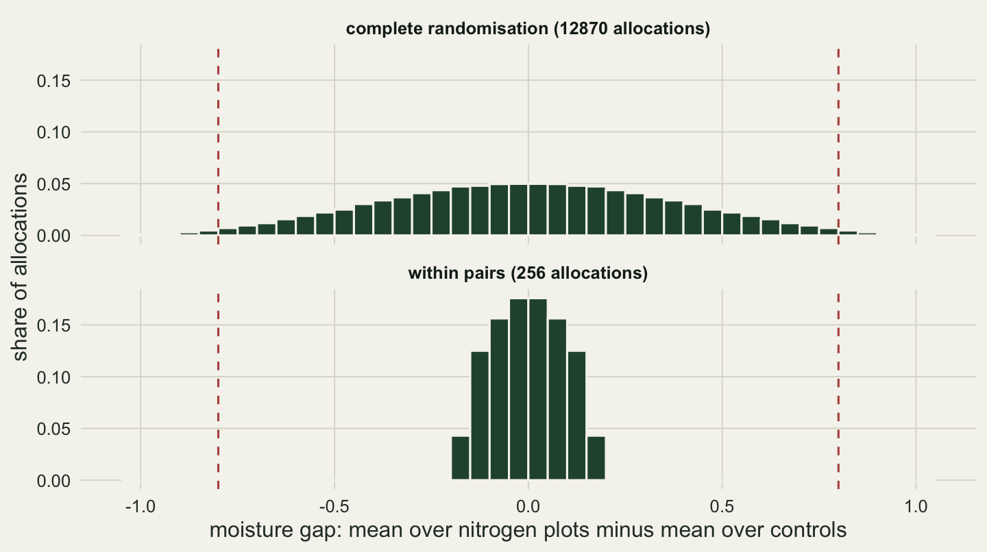
The gap goes into the estimate as extra variance. With independent plot noise, the standard deviation of the estimated nitrogen effect over repeated experiments is the square root of the mean squared gap plus 2 * sd_plot^2 / 8, the textbook variance of a difference between two means of eight. That is the sd_estimate column of the table: 0.509 for complete randomisation and 0.361 within pairs, against 0.350 if there were no gradient at all.
Drawing the paired allocation takes one shuffle per pair. It is the loop from Check four of the design-checking post, with blocks of two:
set.seed(2312)
trt_pairs <- unlist(lapply(1:(n_plot / 2), function(b) sample(c("control", "nitrogen"))))
stopifnot(all(table(pair, trt_pairs) == 1))
plot_id[trt_pairs == "nitrogen"]
[1] 2 4 6 7 10 12 14 16One plot left: sample() on a single number
A second sample() trap turns up in follow-on steps. Say one nitrogen plot in each block should carry a soil-moisture logger, and the script that picks it was written for an earlier layout of four blocks of four plots, with two nitrogen plots per block:
pick_logger <- function(trt, block) {
  vapply(unique(block), function(b) {
    candidates <- plot_id[block == b & trt == "nitrogen"]
    sample(candidates, 1)
  }, numeric(1))
}
set.seed(2313)
nitro_plots <- plot_id[trt_pairs == "nitrogen"]
logger_plot <- pick_logger(trt_pairs, pair)
rbind(nitrogen_plot = nitro_plots, logger_plot = logger_plot)
[,1] [,2] [,3] [,4] [,5] [,6] [,7] [,8]
nitrogen_plot 2 4 6 7 10 12 14 16
logger_plot 2 4 1 1 2 1 10 3expected_right <- sum(1 / nitro_plots)
c(right_plot = sum(logger_plot == nitro_plots), expected = expected_right)right_plot expected
2.000000 1.376786 With pairs, each block holds one nitrogen plot, so candidates is a single number. The R documentation for sample() says what happens then: if x has length 1, is numeric and is at least 1, sampling takes place from 1:x. So sample(14, 1) is not plot 14; it is any whole number from 1 to 14. The same help page gives the fix, a version that always samples from the vector it is given:
set.seed(2314)
draws14  <- replicate(5000, sample(14, 1))
resample <- function(x, ...) x[sample.int(length(x), ...)]
stopifnot(all(draws14 %in% 1:14), setequal(unique(draws14), 1:14),
          all(replicate(200, resample(14, 1)) == 14),
          all(replicate(200, sample("P14", 1)) == "P14"), any(logger_plot != nitro_plots),
          !inherits(tryCatch(sample(14, 1), warning = identity), "warning"))   # nothing warns
c(share_14 = mean(draws14 == 14), exact = 1 / 14)
share_14 exact
0.07500000 0.07142857 sample(14, 1) returned 14 in 0.075 of 5000 draws, against 1/14 exactly. Over the eight pairs the expected number of loggers on the right plot is the sum of 1 over each nitrogen plot number, 1.38, and this run put 2 of 8 where they belong. Nothing warns. Plot identifiers stored as text ("P14") are safe for the same reason: the shortcut only applies to numbers. Either way, one line after the call catches it, stopifnot(all(logger_plot %in% nitro_plots)).
Analyse the pairs as pairs
One season of the paired experiment, analysed three ways:
set.seed(2315)
biomass <- g + rnorm(n_plot, 0, sd_plot) + n_effect * (trt_pairs == "nitrogen")
season  <- data.frame(plot = plot_id, pair = factor(pair), biomass = biomass,
                      treatment = factor(trt_pairs, levels = c("control", "nitrogen")))
d_pair   <- biomass[trt_pairs == "nitrogen"] - biomass[trt_pairs == "control"]
tt_pair  <- t.test(d_pair)                                        # paired t-test
tt_two   <- t.test(biomass[trt_pairs == "nitrogen"], biomass[trt_pairs == "control"],
                   var.equal = TRUE)                              # pairs ignored
aov_pair <- anova(lm(biomass ~ pair + treatment, data = season))  # pair as a block term
stopifnot(isTRUE(all.equal(unname(tt_pair$statistic^2), aov_pair["treatment", "F value"])),
          isTRUE(all.equal(tt_pair$p.value, aov_pair["treatment", "Pr(>F)"])),
          isTRUE(all.equal(unname(tt_pair$estimate), unname(diff(rev(tt_two$estimate))))))
round(rbind(paired    = c(estimate = unname(tt_pair$estimate), se = tt_pair$stderr,
                          df = unname(tt_pair$parameter), p = tt_pair$p.value),
            two_group = c(unname(diff(rev(tt_two$estimate))), tt_two$stderr,
                          unname(tt_two$parameter), tt_two$p.value)), 4)
estimate se df p
paired 1.1695 0.2866 7 0.0047
two_group 1.1695 0.4110 14 0.0130aov_pairAnalysis of Variance Table
Response: biomass
Df Sum Sq Mean Sq F value Pr(>F)
pair 7 7.1605 1.0229 3.1126 0.078598 .
treatment 1 5.4712 5.4712 16.6478 0.004689 **
Residuals 7 2.3005 0.3286
---
Signif. codes: 0 '***' 0.001 '**' 0.01 '*' 0.05 '.' 0.1 ' ' 1The two analyses report the same estimate, 1.170, because in both it is the mean of the nitrogen plots minus the mean of the controls. They differ in the standard error: 0.287 from the within-pair differences on 7 degrees of freedom, against 0.411 from the two-group formula on 14. The p-values are 0.005 and 0.013. The paired t-test and lm() with a pair term are one analysis: the t statistic squared equals the F for treatment, and the p-values agree, which the stopifnot() checks. With blocks of more than two plots, the lm() form is the one that carries over. (t-tests and ANOVA as linear models in R shows why a t-test is a linear model.)
One season shows the mechanism, not how often each analysis finds the effect. For that, the same experiment is repeated twenty thousand times with fresh noise and a fresh allocation each time, under complete randomisation, within pairs, and within four blocks of four plots (two nitrogen per block), and each blocked design is analysed with and without its blocks. The tests are written out by hand so the whole run takes seconds: the two-group t-test, and the lm() test with a block term, which with blocks of two is the paired t-test. A hidden chunk checks both against t.test() and anova(lm()) on one simulated dataset.
two_group_p <- function(y, z) {                       # two-sample pooled t-test
  m1 <- rowSums(y * z) / 8; m0 <- rowSums(y * (1 - z)) / 8
  ss <- rowSums((y - (m1 * z + m0 * (1 - z)))^2)
  se <- sqrt(ss / 14 * (2 / 8))
  cbind(est = m1 - m0, se = se, p = 2 * pt(-abs((m1 - m0) / se), 14))
}
block_p <- function(y, z, blk) {       # lm(y ~ block + treatment), half of each block treated
  nb <- max(blk); df_res <- n_plot - nb - 1
  # residual SS = within-block SS minus treatment SS, which is n_plot / 4 * est^2 when half of each block is treated
  blk_means <- matrix(sapply(1:nb, function(b) rowMeans(y[, blk == b, drop = FALSE])), nrow(y))
  est <- rowSums(y * z) / 8 - rowSums(y * (1 - z)) / 8
  ss_res <- rowSums((y - blk_means[, blk, drop = FALSE])^2) - n_plot / 4 * est^2
  2 * pt(-abs(est / sqrt(ss_res / df_res * (2 / 8))), df_res)
}
block4 <- rep(1:4, each = 4)
run_designs <- function(gmax, effect, nsim) {
  y0 <- matrix(rnorm(nsim * n_plot, 0, sd_plot), nsim) + rep(moisture(gmax), each = nsim)
  z_c <- t(replicate(nsim, sample(rep(0:1, n_plot / 2))))
  z_p <- t(replicate(nsim, as.vector(sapply(1:8, function(b) sample(0:1)))))
  z_4 <- t(replicate(nsim, as.vector(sapply(1:4, function(b) sample(rep(0:1, 2))))))
  y_c <- y0 + effect * z_c; y_p <- y0 + effect * z_p; y_4 <- y0 + effect * z_4
  tg_c <- two_group_p(y_c, z_c); tg_p <- two_group_p(y_p, z_p); tg_4 <- two_group_p(y_4, z_4)
  list(reject = cbind(complete = tg_c[, "p"], pairs_paired = block_p(y_p, z_p, pair), pairs_two_group = tg_p[, "p"],
                      blocks4_block_lm = block_p(y_4, z_4, block4), blocks4_two_group = tg_4[, "p"]) < 0.05,
       sd_est = c(complete = sd(tg_c[, "est"]), pairs = sd(tg_p[, "est"])),
       se_two_group_on_pairs = sqrt(mean(tg_p[, "se"]^2)),
       check = list(y = y_4[1, ], z = z_4[1, ], yp = y_p[1, ], zp = z_p[1, ]))
}
n_sim <- 20000
set.seed(2316)
power_run <- run_designs(grad_max, n_effect, n_sim)
set.seed(2317)
null_run  <- run_designs(grad_max, 0, n_sim)
rates <- rbind(power = colMeans(power_run$reject), size = colMeans(null_run$reject))
mc_se <- sqrt(rates * (1 - rates) / n_sim)
round(rbind(rates, se_power = mc_se["power", ], se_size = mc_se["size", ]), 4)
complete pairs_paired pairs_two_group blocks4_block_lm
power 0.3044 0.4757 0.2299 0.4756
size 0.0499 0.0511 0.0056 0.0489
se_power 0.0033 0.0035 0.0030 0.0035
se_size 0.0015 0.0016 0.0005 0.0015
blocks4_two_group
power 0.2450
size 0.0093
se_power 0.0030
se_size 0.0007round(c(power_run$sd_est, se_reported_two_group_on_pairs = power_run$se_two_group_on_pairs), 3) complete pairs
0.510 0.359
se_reported_two_group_on_pairs
0.519 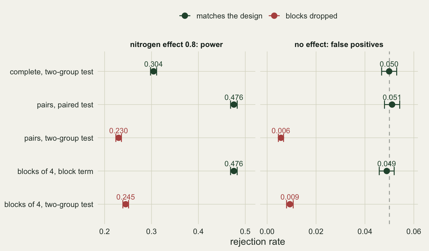
Pairing raised the power from 0.304 under complete randomisation to 0.476 with the paired test, with Monte Carlo standard errors of at most 0.004. The same paired allocations, analysed as two independent groups, found the effect in 0.230 of experiments: less than the paired test, and, on this gradient, less than not pairing at all. Blocks of four behave the same way, 0.476 with the block term and 0.245 without.
The reason sits in the two standard deviations printed above. Pairing made the estimate more precise: its spread over repeated experiments fell from 0.510 to 0.359, matching the exact values listed earlier. The two-group test does not know that. It computes its standard error from the spread of plots within each group, and with the gradient in that spread it reports 0.519 (root mean square over the simulated experiments): a figure close to the spread of the complete design’s estimate, attached to an estimate that is far more precise. So the test is too cautious. With no nitrogen effect it rejected 0.006 of the time instead of 0.05, while the paired test held 0.051. This is the reverse of pseudoreplication: no false positives are added, but everything the pairing earned is thrown away, and on this gradient a little more. None of it is new; the paired t-test is the two-treatment case of the randomised block analysis (Quinn and Keough 2002), and the simulation only puts numbers on what leaving the blocks out does in this layout.
How much pairing buys depends on the gradient
The gain above belongs to one layout. It comes entirely from the gradient: pairing removes the part of the plot-to-plot differences that neighbouring plots share, so it can only help as much as neighbours are alike. Running the same comparison over gradients from none to twice the one above, with the noise fixed at 0.7:
grad_values <- c(0, 0.5, 1, 1.5, 2, 2.5, 3.5, 5)
n_sweep <- 10000; sweep_se <- sqrt(0.25 / n_sweep)    # largest possible Monte Carlo SE of a rate
set.seed(2318)
sweep <- t(sapply(grad_values, function(gm) colMeans(run_designs(gm, n_effect, n_sweep)$reject)))
sweep <- data.frame(grad_max = grad_values, sweep)
round(sweep[, c("grad_max", "complete", "pairs_paired", "pairs_two_group")], 3)
grad_max complete pairs_paired pairs_two_group
1 0.0 0.566 0.502 0.566
2 0.5 0.549 0.503 0.550
3 1.0 0.494 0.503 0.492
4 1.5 0.433 0.499 0.415
5 2.0 0.365 0.487 0.320
6 2.5 0.312 0.474 0.234
7 3.5 0.215 0.452 0.093
8 5.0 0.141 0.413 0.013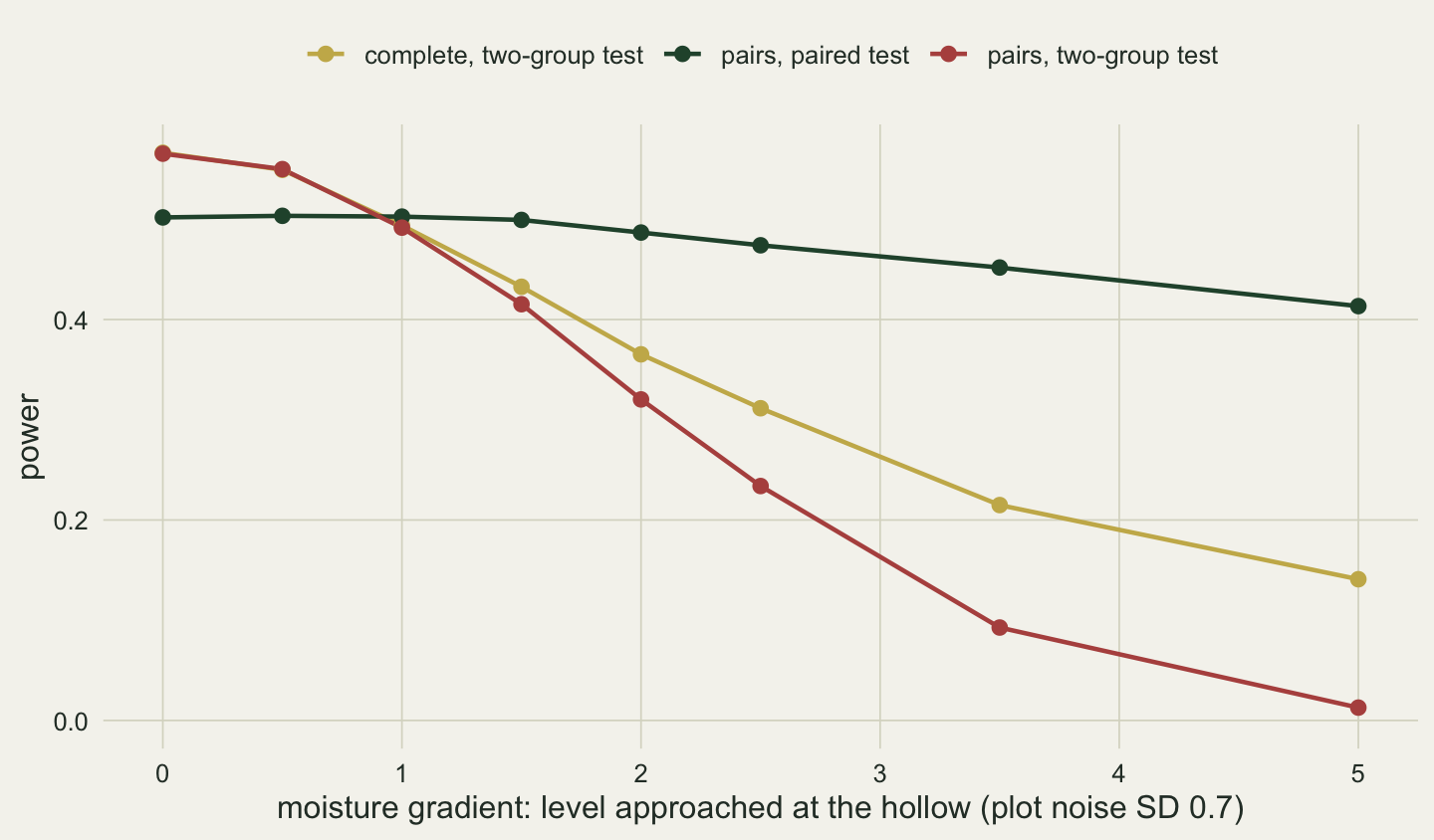
With no gradient at all, pairing costs power: the paired test has 0.502 against 0.566 for complete randomisation, because it spends half its degrees of freedom (7 instead of 14) on pairs that are no more alike than any two plots. In that case the two-group test on paired plots is not a mistake that costs anything; it gives 0.566, higher than the paired test. At a gradient of 1 unit the two designs are level (0.503 paired against 0.494 complete). As the gradient steepens, the complete design loses power, the paired test keeps most of it (0.413 at a gradient of 5 units, against 0.141), and the two-group test on paired plots collapses to 0.013. That test matches complete randomisation up to a gradient of 1 (0.492 against 0.494 at 1) and is clearly below it from 2 on (0.320 against 0.365 at 2), and at no gradient in this sweep did it beat complete randomisation by more than Monte Carlo noise. The cost of dropping the pairs comes from the gradient, like the gain from keeping them. Legendre et al. (2004) reach the practical conclusion from a much wider set of simulated field surfaces: where the response has spatial structure, block the layout and put the blocks in the analysis.
What to check in your own experiment
Count the groups after every allocation, table(trt), and make the script stop if the counts are not the ones you planned. Draw with sample() on a vector that holds the labels in the numbers you want; replace = TRUE is for coin tossing, not for allocation.
Store the allocation as a column in the data file before the field work starts. The seed alone reproduces it only on an R that samples the same way.
Look for sample(x, 1) or sample(x) where x is a vector of plot numbers that could shrink to a single element. Use x[sample.int(length(x), 1)], or store plot IDs as text, and check afterwards that every pick is in x.
Before you analyse, write down the unit that each coin toss was applied within: pairs, blocks, or the whole site. That unit belongs in the model, as a paired test or a block term in lm(). A quick check is the residual degrees of freedom: sixteen plots in eight pairs give 7 for the treatment test. A test on 14 has dropped the pairs.
Decide whether to pair before the season, from what you know about the site. Pairs pay for themselves only if neighbouring plots are more alike than plots in general; on a site with no gradient in the response they cost degrees of freedom.
Honest limits
The simulation has one layout: a single row of sixteen plots, one smooth gradient, independent normal noise, and a nitrogen effect that is the same everywhere. Where the effect itself changes along the gradient, a pair or block term handles the baseline differences but not the interaction, and eight pairs cannot estimate much of one. Patchy or spatially autocorrelated variation that does not follow the pairs is not simulated here; Legendre et al. (2004) do that. The power figures belong to these constants and would differ for another site. The analyses are t-tests and linear models; a randomisation test, which takes its null distribution from the allocations listed earlier, is another valid analysis of the same design and is not covered.
References
Hurlbert SH 1984 Ecological Monographs 54(2):187-211 (10.2307/1942661)
Legendre P, Dale MRT, Fortin MJ, Casgrain P, Gurevitch J 2004 Ecology 85(12):3202-3214 (10.1890/03-0677)
Quinn GP, Keough MJ 2002 Experimental Design and Data Analysis for Biologists (ISBN 9780521009768)
R Core Team 2024 R documentation: Random Samples and Permutations, sample (https://stat.ethz.ch/R-manual/R-devel/library/base/html/sample.html)
R Core Team 2024 R documentation: Random Number Generation, RNGkind (https://stat.ethz.ch/R-manual/R-devel/library/base/html/Random.html)