library(ggplot2)

te_paper  <- "#f5f4ee"
te_ink    <- "#16241d"
te_body   <- "#2c3a31"
te_forest <- "#275139"
te_rust   <- "#b5534e"
te_gold   <- "#c9b458"
te_line   <- "#dad9ca"

theme_datasheet <- function() {
  theme_minimal(base_size = 12) +
    theme(plot.background  = element_rect(fill = te_paper, colour = NA),
          panel.background = element_rect(fill = te_paper, colour = NA),
          panel.grid.major = element_line(colour = te_line, linewidth = 0.3),
          panel.grid.minor = element_blank(),
          text             = element_text(colour = te_body),
          plot.title       = element_text(colour = te_ink, face = "bold"),
          plot.subtitle    = element_text(colour = te_body),
          axis.text        = element_text(colour = te_body))
}

fmt_e <- function(x) formatC(x, format = "e", digits = 2)Seasonal matrix models and the census date
R
population dynamics
matrix models
demography
conservation
ecology tutorial
Lambda from a seasonal matrix model does not depend on the census date, but the annual matrix and its elasticities do. Periodic sensitivity analysis in R.
A hay meadow perennial is monitored by two teams. One counts seedlings, non-flowering rosettes and flowering plants in the first week of April, before growth starts. The other counts the same three stages at midsummer, just before the seed is shed, because that is when flowering plants are easiest to find. Both teams follow marked plants for several years, both build a stage matrix from one census to the next, and both report an elasticity analysis to the reserve manager. The two reports disagree about how much seed production matters. Neither team has made an arithmetic mistake.
The reason is that the plant does not live in annual steps. Rosettes grow and bolt in spring, flowering plants set seed and many die back to rosettes in summer, the hay cut knocks flowering stems back in autumn, and seedlings die in the frost. A year is the product of four seasonal transitions, and an annual matrix is that product read from one particular starting point. This post builds the four seasonal matrices, multiplies them from each of the four possible census dates, and measures what survives the change of starting point and what does not.
It sits between two existing posts. Leslie matrix population models in R builds an age matrix for a census taken just before breeding, where the fertility entry in the top row is survival of the newborns times fecundity, p0 * m_age. A census just after breeding would put the survival factor in a different place, and the pre-breeding versus post-breeding choice is the two-season case of everything below. Sensitivity and elasticity of matrix models computes elasticities of one annual stage matrix and sums them by process to decide between adult survival and seed output. Here the question is whether that sum is a property of the plant or of the week the census was taken. The periodic sensitivity formula of Caswell and Trevisan is the tool that separates the two.
Four seasons, one year
The model has three stages at every census: seedlings, vegetative rosettes and flowering plants. Each seasonal matrix is a survival step followed by a movement step, and summer also adds seedlings. Every rate below is a design constant written down before any eigenvalue was computed; the recruitment rate of five seedlings per flowering plant is the only one chosen with the growth rate in mind, so that the population declines slowly rather than crashing, and none of them was changed after the results were seen.
stage_names  <- c("seedling", "rosette", "flowering")
season_names <- c("spring", "summer", "autumn", "winter")
n_stage  <- length(stage_names)
n_season <- length(season_names)

# survival through each season, by stage
surv <- rbind(spring = c(0.75, 0.90, 0.95),
              summer = c(0.80, 0.95, 0.90),
              autumn = c(0.75, 0.95, 0.95),
              winter = c(0.55, 0.92, 0.90))
grow_sr  <- 0.40  # seedling to rosette, spring
bolt_rf  <- 0.35  # rosette to flowering, spring
back_spr <- 0.05  # flowering back to rosette, spring
back_sum <- 0.45  # flowering back to rosette after seeding, summer
back_aut <- 0.15  # flowering back to rosette after the hay cut, autumn
recruits <- 5     # seedlings per flowering plant counted at the start of summer

move_mat <- function(to_ros = 0, to_flw = 0, to_back = 0) {
  matrix(c(1 - to_ros, 0,          0,
           to_ros,     1 - to_flw, to_back,
           0,          to_flw,     1 - to_back),
         n_stage, n_stage, byrow = TRUE)
}
fec_mat <- matrix(0, n_stage, n_stage)
fec_mat[1, 3] <- recruits

season_mat <- list(
  spring = move_mat(grow_sr, bolt_rf, back_spr) %*% diag(surv["spring", ]),
  summer = move_mat(to_back = back_sum) %*% diag(surv["summer", ]) + fec_mat,
  autumn = move_mat(to_back = back_aut) %*% diag(surv["autumn", ]),
  winter = move_mat() %*% diag(surv["winter", ]))
A census at the start of season h sees the plant go through season h first and season h - 1 last, so the annual matrix for that census is the product with the first season on the right. Written for a spring census it is winter times autumn times summer times spring. The other three census dates give the same four factors in rotated order.
season_order <- function(h) ((h - 1):(h + n_season - 2)) %% n_season + 1
chain_prod <- function(idx) {
  out <- diag(n_stage)
  for (k in idx) out <- season_mat[[k]] %*% out
  out
}
annual_at <- function(h) chain_prod(season_order(h))

lead_eig <- function(a_mat) {
  e_r <- eigen(a_mat)
  i_r <- which.max(Re(e_r$values))
  w_r <- Re(e_r$vectors[, i_r])
  w_r <- w_r / sum(w_r)
  e_l <- eigen(t(a_mat))
  v_l <- Re(e_l$vectors[, which.max(Re(e_l$values))])
  v_l <- v_l / sum(v_l * w_r)
  list(lambda = Re(e_r$values[i_r]), w = w_r, v = v_l, sens = outer(v_l, w_r))
}

annual_list <- lapply(seq_len(n_season), annual_at)
eig_list    <- lapply(annual_list, lead_eig)
lam_phase   <- vapply(eig_list, function(e) e$lambda, 0)
lam_spread  <- max(lam_phase) - min(lam_phase)
spec_sorted <- sapply(annual_list, function(a) sort(Mod(eigen(a)$values)))
spec_gap    <- max(apply(spec_sorted, 1, function(r) max(r) - min(r)))
lam_rev     <- lead_eig(chain_prod(rev(season_order(1))))$lambda
The growth rate is 0.980561 from the spring census, 0.980561 from summer, 0.980561 from autumn and 0.980561 from winter. The largest difference between the four is 2.11e-15, and the largest difference in the modulus of any of the three eigenvalues is 2.11e-15: rounding error, nothing else.
This is a theorem and not a property of these rates. For square matrices X and Y the products XY and YX have the same characteristic polynomial, and a rotation of a product of four factors is a repeated application of that fact. The census date cannot change lambda, whatever the seasons are.
The order of the factors is a different matter. Multiplying the seasons in calendar order from the left, spring times summer times autumn times winter, is not a rotation of the correct product but its reversal, and it is an easy line of code to write by accident. That product has a dominant eigenvalue of 1.1015 against the correct 0.9806: a declining population turned into a growing one. The starting season is free; the direction of travel is not.
The stable stage distribution belongs to a date
w_phase <- sapply(eig_list, function(e) e$w)
dimnames(w_phase) <- list(stage_names, season_names)
seed_share <- w_phase["seedling", ]
flow_share <- w_phase["flowering", ]

# one season carries the stable structure of one census to the next
prop_gap <- max(vapply(seq_len(n_season), function(h) {
  nxt <- season_mat[[h]] %*% w_phase[, h]
  max(abs(nxt / sum(nxt) - w_phase[, h %% n_season + 1]))
}, 0))

# and a long seasonal projection from an arbitrary start ends there
n_years   <- 40
n_now     <- c(100, 100, 100)
last_frac <- matrix(0, n_stage, n_season)
for (yr in seq_len(n_years)) for (h in seq_len(n_season)) {
  if (yr == n_years) last_frac[, h] <- n_now / sum(n_now)
  n_now <- season_mat[[h]] %*% n_now
}
proj_gap <- max(abs(last_frac - w_phase))
The right eigenvectors are not shared. Seedlings make up 0.499 of the stable population at the April census, 0.271 at midsummer before the new seed has germinated, 0.678 at the start of autumn once the summer cohort is in, and 0.624 at the start of winter. Flowering plants run from 0.056 to 0.243. The four vectors are linked: pushing the stable vector of one census through the next seasonal matrix and renormalising gives the stable vector of the following census, to within 3.89e-16. A forty year seasonal projection from an equal start lands on all four within 3.89e-16, so these are the structures a real population would show.
For monitoring this is the familiar part. A stable structure is only comparable with an observed one taken at the same point in the year, and a stage vector from a midsummer count cannot be checked against a stable distribution computed from an April matrix.
stable_df <- data.frame(
  census = factor(rep(season_names, each = n_stage), levels = season_names),
  stage  = factor(rep(stage_names, n_season), levels = rev(stage_names)),
  share  = as.vector(w_phase))

ggplot(stable_df, aes(census, share, fill = stage)) +
  geom_col(width = 0.65, colour = te_paper, linewidth = 0.4) +
  geom_text(aes(label = sprintf("%.2f", share), colour = stage),
            position = position_stack(vjust = 0.5), size = 3.6,
            show.legend = FALSE) +
  scale_colour_manual(values = c(seedling = te_ink, rosette = te_paper,
                                 flowering = te_paper), guide = "none") +
  scale_fill_manual(values = c(seedling = te_gold, rosette = te_forest,
                               flowering = te_rust),
                    breaks = stage_names, name = NULL) +
  labs(x = "census taken at the start of", y = "share of the stable population",
       title = "One plant, four stable structures",
       subtitle = "lambda is the same at every census; the eigenvector is not") +
  theme_datasheet() +
  theme(legend.position = "bottom")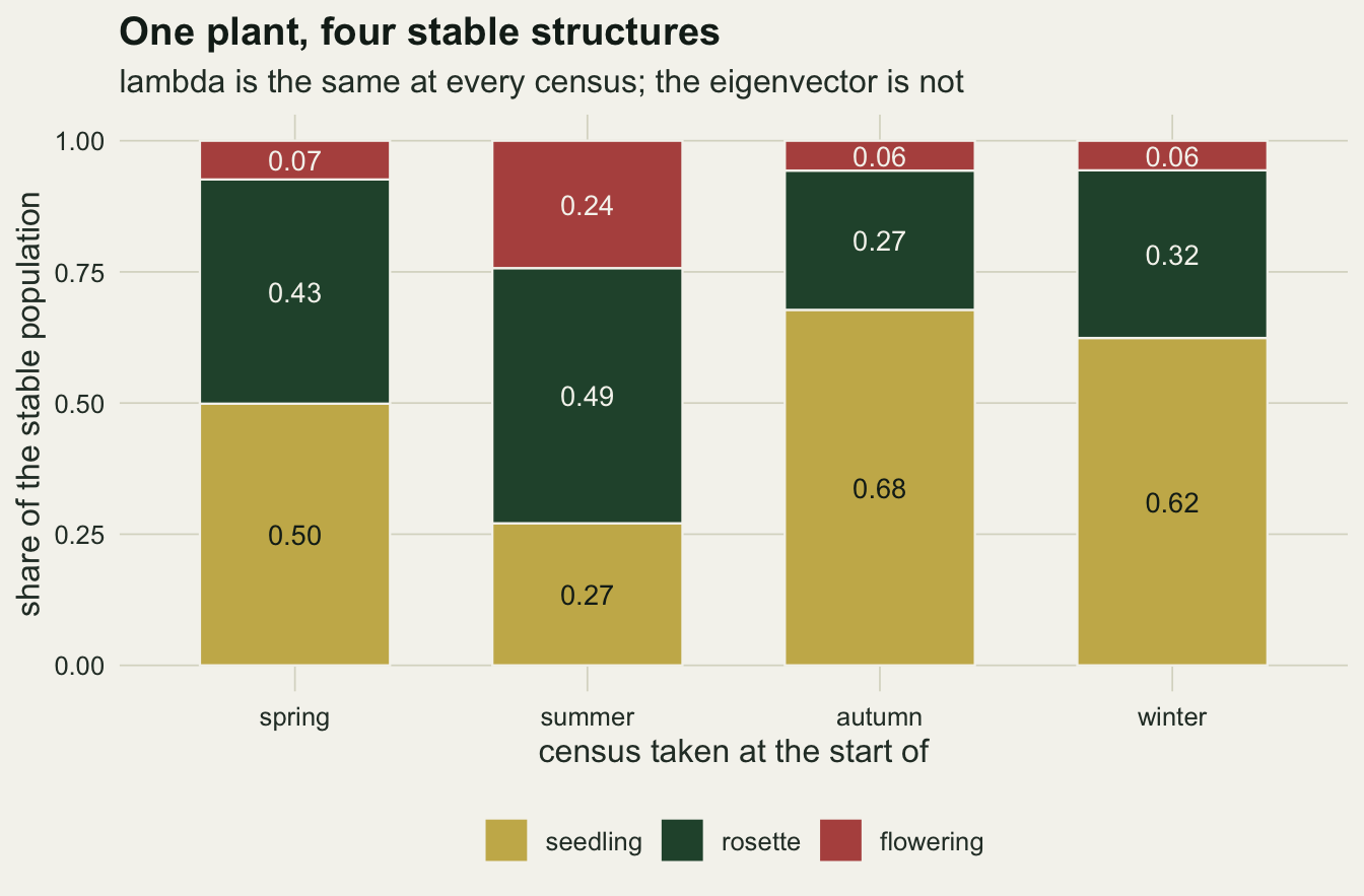
Annual elasticities depend on the census date
The next step in most reports is an elasticity analysis of the annual matrix, with elasticity in the sense of de Kroon and colleagues: the proportional change in lambda for a proportional change in one entry, so that the entries of one matrix sum to one. The entries are classified here into four processes: the diagonal is stasis, moves to a larger stage are progression, the top row away from the diagonal is reproduction, and flowering back to rosette is retrogression. A three-way split that lumps retrogression with stasis, which is also common, would count the summer retrogression entry as survival.
elas_annual <- lapply(seq_len(n_season), function(h)
  annual_list[[h]] * eig_list[[h]]$sens / eig_list[[h]]$lambda)

proc_class <- matrix(c("stasis",      "reproduction", "reproduction",
                       "progression", "stasis",       "retrogression",
                       "progression", "progression",  "stasis"),
                     n_stage, n_stage, byrow = TRUE)
entry_lab <- outer(stage_names, stage_names,
                   function(to, from) paste(from, "to", to))

top_entry  <- vapply(elas_annual, function(e) entry_lab[which.max(e)], "")
top_val    <- vapply(elas_annual, max, 0)
second_val <- vapply(elas_annual, function(e) sort(e, decreasing = TRUE)[2], 0)
second_lab <- vapply(elas_annual, function(e)
  entry_lab[order(e, decreasing = TRUE)[2]], "")
n_nonzero  <- vapply(annual_list, function(a) sum(a > 1e-12), 0)

proc_share <- sapply(elas_annual, function(e) tapply(e, proc_class, sum))
colnames(proc_share) <- season_names

# rotating the census by one season is a similarity transform
sim_gap <- max(vapply(seq_len(n_season), function(h) {
  max(abs(season_mat[[h]] %*% annual_list[[h]] %*% solve(season_mat[[h]]) -
            annual_list[[h %% n_season + 1]]))
}, 0))
elas_gap <- function(h1, h2) max(abs(elas_annual[[h1]] - elas_annual[[h2]]))
gap_win_spr <- elas_gap(4, 1)
gap_aut_win <- elas_gap(3, 4)
gap_spr_sum <- elas_gap(1, 2)
gap_sum_aut <- elas_gap(2, 3)

# how much of the midsummer 'flowering to rosette' entry is recruitment
after_sum     <- chain_prod(c(3, 4, 1))
retro_total   <- annual_list[[2]][2, 3]
retro_recruit <- after_sum[2, 1] * recruits

# does a small change in one design rate swap the two leading midsummer entries?
build_seasons <- function(rate_set, surv_set) {
  fec_p <- matrix(0, n_stage, n_stage)
  fec_p[1, 3] <- rate_set[["recruits"]]
  list(move_mat(rate_set[["grow_sr"]], rate_set[["bolt_rf"]], rate_set[["back_spr"]]) %*%
         diag(surv_set["spring", ]),
       move_mat(to_back = rate_set[["back_sum"]]) %*% diag(surv_set["summer", ]) + fec_p,
       move_mat(to_back = rate_set[["back_aut"]]) %*% diag(surv_set["autumn", ]),
       move_mat() %*% diag(surv_set["winter", ]))
}
summer_top <- function(s_list) {
  a_sum <- s_list[[1]] %*% s_list[[4]] %*% s_list[[3]] %*% s_list[[2]]
  e_sum <- lead_eig(a_sum)
  entry_lab[which.max(a_sum * e_sum$sens / e_sum$lambda)]
}
rate_base <- c(grow_sr = grow_sr, bolt_rf = bolt_rf, back_spr = back_spr,
               back_sum = back_sum, back_aut = back_aut, recruits = recruits)
rate_desc <- c(grow_sr = "seedling to rosette rate", bolt_rf = "rosette to flowering rate",
               back_spr = "spring flowering to rosette rate",
               back_sum = "summer flowering to rosette rate",
               back_aut = "autumn flowering to rosette rate",
               recruits = "recruitment rate")
step_prob  <- 0.02  # added to or taken from one probability at a time
step_recr  <- 0.2   # added to or taken from seedlings per flowering plant
rebuild_gap <- max(mapply(function(x, y) max(abs(x - y)),
                          build_seasons(rate_base, surv), season_mat))
swap_hits <- character(0)
swap_new  <- character(0)
n_perturb <- 0
for (nm in names(rate_base)) for (sgn in c(-1, 1)) {
  rate_new <- rate_base
  rate_new[nm] <- rate_base[nm] + sgn * ifelse(nm == "recruits", step_recr, step_prob)
  n_perturb <- n_perturb + 1
  top_new <- summer_top(build_seasons(rate_new, surv))
  if (top_new != top_entry[2]) {
    swap_hits <- c(swap_hits, paste(rate_desc[nm], ifelse(sgn < 0, "lower", "higher")))
    swap_new  <- c(swap_new, top_new)
  }
}
for (h in seq_len(n_season)) for (j in seq_len(n_stage)) for (sgn in c(-1, 1)) {
  surv_new <- surv
  surv_new[h, j] <- surv[h, j] + sgn * step_prob
  n_perturb <- n_perturb + 1
  top_new <- summer_top(build_seasons(rate_base, surv_new))
  if (top_new != top_entry[2]) {
    swap_hits <- c(swap_hits, paste(season_names[h], stage_names[j], "survival",
                                    ifelse(sgn < 0, "lower", "higher")))
    swap_new  <- c(swap_new, top_new)
  }
}
n_swap <- length(swap_hits)
swap_to  <- paste(unique(swap_new), collapse = " or ")
From the April census the largest annual elasticity is on rosette to rosette, at 0.392. From the midsummer census it is on rosette to flowering, at 0.251, with rosette to rosette second at 0.246. The headline entry changes, but only just: in the summer matrix the two leading entries differ by 0.005. The order survives most small changes, though not all: moving one design rate at a time, each probability up or down by 0.02 and recruitment by 0.2 seedlings, gives 36 perturbed models, and 2 of them put rosette to rosette back on top (rosette to flowering rate lower; summer rosette survival higher). The winter and autumn censuses both put rosette to rosette first. Even the list of transitions changes: the summer census matrix has 7 nonzero entries and the other three have 8, because a rosette counted at midsummer cannot bolt until the following spring, so the seed it eventually sets is shed after the next census and the rosette to seedling entry is zero.
The process sums move much more than the top entry does. Reproduction carries 0.185 of the elasticity in the April matrix and 0.028 in the midsummer matrix, while retrogression goes from 0.046 to 0.223. The midsummer team would tell the manager that seed production barely matters and that flowering plants falling back to rosettes matters a great deal; the April team would put the same two processes in the opposite order.
Neither label is wrong about its own matrix. At a midsummer census, a flowering plant sets seed straight after being counted, and the seedlings that grow into rosettes the next spring are counted as rosettes a year later. Of the midsummer entry labelled “flowering to rosette”, 0.881, the part that runs through recruitment and growth is 0.619, a share of 0.70; flowering plants actually shrinking supply the rest. The biological process behind an annual entry depends on which seasons it spans.
There is a precise rule for when two census dates agree. Moving the census forward one season turns the annual matrix A into B A B^-1, where B is the matrix of the season skipped, and this identity holds here to 8.88e-16. A similarity transform keeps every eigenvalue but in general not the elasticities, unless B is diagonal, in which case each annual entry is only rescaled by a ratio of survivals and its elasticity does not move. Winter in this model is pure survival, and the winter and spring census elasticities differ by at most 5.00e-16. Autumn includes the hay cut that sends flowering plants back to rosettes, and the autumn and winter census elasticities differ by up to 0.025. Skipping spring, the season in which seedlings grow and rosettes bolt, gives the largest single difference, 0.177, and skipping summer, with its recruitment and dieback, gives 0.172.
elas_df <- do.call(rbind, lapply(seq_len(n_season), function(h) {
  data.frame(census = factor(season_names[h], levels = season_names),
             to     = factor(rep(stage_names, n_stage), levels = rev(stage_names)),
             from   = factor(rep(stage_names, each = n_stage), levels = stage_names),
             elas   = as.vector(elas_annual[[h]]),
             top    = as.vector(elas_annual[[h]] == max(elas_annual[[h]])))
}))
elas_df$census <- factor(paste(elas_df$census, "census"),
                         levels = paste(season_names, "census"))

ggplot(elas_df, aes(from, to, fill = elas)) +
  geom_tile(colour = te_paper, linewidth = 1.2) +
  geom_tile(data = elas_df[elas_df$top, ], fill = NA,
            colour = te_rust, linewidth = 1.3) +
  geom_text(aes(label = sprintf("%.3f", elas),
                colour = elas > 0.2), size = 3.7) +
  scale_fill_gradient(low = te_paper, high = te_forest, name = "elasticity") +
  scale_colour_manual(values = c(`FALSE` = te_ink, `TRUE` = te_paper),
                      guide = "none") +
  facet_wrap(~ census, ncol = 2) +
  labs(x = "from stage", y = "to stage",
       title = "Same plant, four elasticity matrices",
       subtitle = "winter and spring censuses agree because winter is pure survival") +
  theme_datasheet() +
  theme(panel.grid.major = element_blank(),
        strip.text = element_text(colour = te_ink, face = "bold"),
        legend.position = "bottom")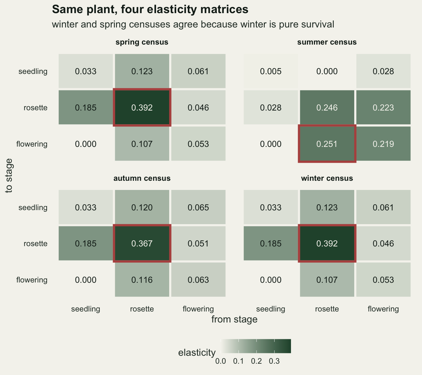
Elasticities to seasonal rates do not
The way out is to stop asking about entries of an annual matrix and ask about entries of the seasonal matrices, which are the rates the plant actually has. Caswell and Trevisan gave the sensitivity of lambda to an entry of season h, and Caswell’s textbook covers it among its time-varying models. Write the annual matrix for a census at the start of season h as A = P B_h, where P is the product of the other three seasons in their order. Then a small change dB_h changes A by P dB_h, and the chain rule turns the ordinary sensitivity matrix of A, S_A = v w' with v'w = 1, into
S_Bh = t(P) %*% S_A.
The same argument works from any census date, not only the one that starts season h. If the seasons applied before h in that year are R and those applied after are L, then A = L B_h R and the sensitivity is t(L) %*% S_A %*% t(R). The chunk below computes all sixteen combinations of season and census, checks the Caswell and Trevisan form against them, and checks the result against a brute force perturbation of every nonzero seasonal entry.
seasonal_sens <- function(k, h) {
  idx    <- season_order(h)
  pos    <- which(idx == k)
  before <- chain_prod(idx[seq_len(pos - 1)])
  after  <- chain_prod(idx[-seq_len(pos)])
  t(after) %*% eig_list[[h]]$sens %*% t(before)
}
sens_route <- lapply(seq_len(n_season), function(k)
  lapply(seq_len(n_season), function(h) seasonal_sens(k, h)))

route_gap <- max(sapply(seq_len(n_season), function(k)
  max(sapply(sens_route[[k]], function(s_m) max(abs(s_m - sens_route[[k]][[k]]))))))
ct_gap <- max(sapply(seq_len(n_season), function(k) {
  p_rest <- chain_prod(season_order(k)[-1])
  max(abs(t(p_rest) %*% eig_list[[k]]$sens - sens_route[[k]][[1]]))
}))

step_fd <- 1e-6
fd_gap  <- 0
for (k in seq_len(n_season)) for (i in seq_len(n_stage)) for (j in seq_len(n_stage)) {
  if (season_mat[[k]][i, j] == 0) next
  keep <- season_mat[[k]]
  season_mat[[k]][i, j] <- keep[i, j] + step_fd
  lam_up <- lead_eig(annual_at(1))$lambda
  season_mat[[k]] <- keep
  fd_now <- (lam_up - lam_phase[1]) / step_fd
  fd_gap <- max(fd_gap, abs(fd_now - sens_route[[k]][[1]][i, j]))
}

elas_season <- lapply(seq_len(n_season), function(k)
  season_mat[[k]] * sens_route[[k]][[1]] / lam_phase[1])
season_sums <- vapply(elas_season, sum, 0)
Across all sixteen routes the seasonal sensitivities agree to 2.00e-15, the Caswell and Trevisan form matches them to 1.33e-15, and the finite difference check agrees to 5.83e-07, which is consistent with the truncation error of a one-sided difference with a step of a millionth. The elasticities of each seasonal matrix sum to one separately: 1.000000, 1.000000, 1.000000 and 1.000000, because lambda scales in proportion to every factor of the product.
The routes agree for a plain reason, which is neither a numerical accident nor a deep result. Lambda is one function of the four seasonal matrices, and the census date is not one of its arguments; its derivative with respect to a spring entry therefore cannot depend on the census date. The formula is what makes that derivative cheap to compute. What does depend on the census is the annual matrix, which is a derived object, and the derivatives of lambda with respect to its entries.
What a manager can act on
A manager cannot change an entry of an annual matrix. What a manager can change is closer to a seasonal rate: winter survival of rosettes under a different grazing regime, or summer recruitment, which a hay cut brought forward into summer, before the seed is shed, would reduce. Here survival of stage j through season h multiplies column j of that season’s matrix, apart from the recruitment entry, so its elasticity is a column sum of the seasonal elasticities. Recruitment is the single summer entry for seedlings per flowering plant.
rate_tab <- do.call(rbind, lapply(seq_len(n_season), function(h) {
  do.call(rbind, lapply(seq_len(n_season), function(k) {
    e_k    <- season_mat[[k]] * sens_route[[k]][[h]] / lam_phase[h]
    surv_e <- colSums(e_k)
    if (k == 2) surv_e[3] <- surv_e[3] - e_k[1, 3]
    out <- data.frame(route = season_names[h],
                      rate  = paste(season_names[k], stage_names, "survival"),
                      elas  = surv_e)
    if (k == 2) out <- rbind(out, data.frame(route = season_names[h],
                                             rate  = "summer recruitment",
                                             elas  = e_k[1, 3]))
    out
  }))
}))
rate_gap <- max(tapply(rate_tab$elas, rate_tab$rate, function(x) max(x) - min(x)))
rate_one <- rate_tab[rate_tab$route == "spring", ]
rate_one <- rate_one[order(rate_one$elas, decreasing = TRUE), ]
e_recruit <- rate_one$elas[rate_one$rate == "summer recruitment"]
rank_recruit <- which(rate_one$rate == "summer recruitment")
n_rates <- nrow(rate_one)
repro_ratio <- proc_share["reproduction", "spring"] / proc_share["reproduction", "summer"]
w_rosette_spr <- eig_list[[1]]$v[2] * eig_list[[1]]$w[2]
seed_tie_rates <- paste(c("spring", "autumn", "winter"), "seedling survival")
e_seed_tie   <- rate_one$elas[rate_one$rate == "autumn seedling survival"]
seed_tie_gap <- max(abs(rate_one$elas[rate_one$rate %in% seed_tie_rates] - e_seed_tie))
Computed from each of the four census routes, the 13 rate elasticities differ by at most 1.44e-15. The largest is winter rosette survival at 0.623, tied with spring rosette survival at 0.623, then autumn rosette survival at 0.603 and summer rosette survival at 0.497. Recruitment ranks 9 of 13, with an elasticity of 0.185.
The ties are exact and have a short explanation. The elasticity of lambda to a survival rate that multiplies a whole column equals the product of reproductive value and stable abundance for that stage at the census that opens the season, v_j w_j, which for rosettes at the April census is 0.623. Winter is survival only, with no movement into or out of any stage, so v_j w_j is the same at the start of winter and at the start of spring for all three stages, and each stage’s winter and spring survival rates tie. Autumn moves no seedlings in or out either, so autumn seedling survival joins that tie: spring, autumn and winter seedling survival all have elasticity 0.218, equal to within 1.67e-16.
Now compare the process sums of the two annual matrices with the recruitment elasticity. The April matrix put 0.185 on reproduction, which is the recruitment elasticity itself, because the two off-diagonal top row entries of that matrix consist entirely of paths through summer recruitment, and no other entry contains one. The midsummer matrix put 0.028 there, 6.6 times less, because most of the recruitment in that matrix is hidden in an entry labelled retrogression. The management answer that does not move with the census is the one phrased in seasonal rates: rosette survival first, recruitment well down the list but not negligible.
rate_tab$rate  <- factor(rate_tab$rate, levels = rev(rate_one$rate))
rate_tab$route <- factor(rate_tab$route, levels = season_names)

ggplot(rate_tab, aes(elas, rate, colour = route, shape = route)) +
  geom_point(size = 2.4, position = position_dodge(width = 0.7)) +
  scale_colour_manual(values = c(te_forest, te_rust, te_gold, te_ink),
                      name = "census used") +
  scale_shape_manual(values = c(16, 17, 15, 18), name = "census used") +
  scale_x_continuous(limits = c(0, NA)) +
  labs(x = "elasticity of lambda", y = NULL,
       title = "Seasonal rates give one answer",
       subtitle = "four census routes, one set of values") +
  theme_datasheet() +
  theme(legend.position = "bottom")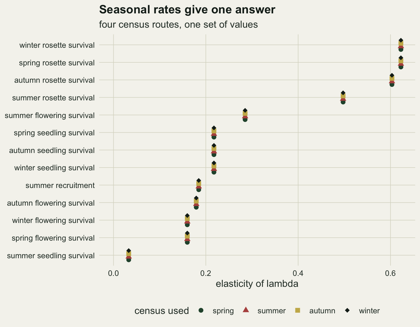
proc_df <- data.frame(
  census  = factor(rep(season_names, each = nrow(proc_share)), levels = season_names),
  process = factor(rep(rownames(proc_share), n_season),
                   levels = c("stasis", "progression", "reproduction", "retrogression")),
  share   = as.vector(proc_share))

ggplot(proc_df, aes(census, share, fill = process)) +
  geom_col(position = position_dodge(width = 0.8), width = 0.75,
           colour = te_body, linewidth = 0.25) +
  geom_hline(yintercept = e_recruit, linetype = "dashed",
             colour = te_ink, linewidth = 0.6) +
  scale_fill_manual(values = c(stasis = te_forest, progression = te_line,
                               reproduction = te_gold, retrogression = te_rust),
                    name = NULL) +
  labs(x = "census taken at the start of", y = "summed elasticity",
       title = "The process sums follow the calendar",
       subtitle = "dashed line: elasticity of lambda to summer recruitment") +
  theme_datasheet() +
  theme(legend.position = "bottom")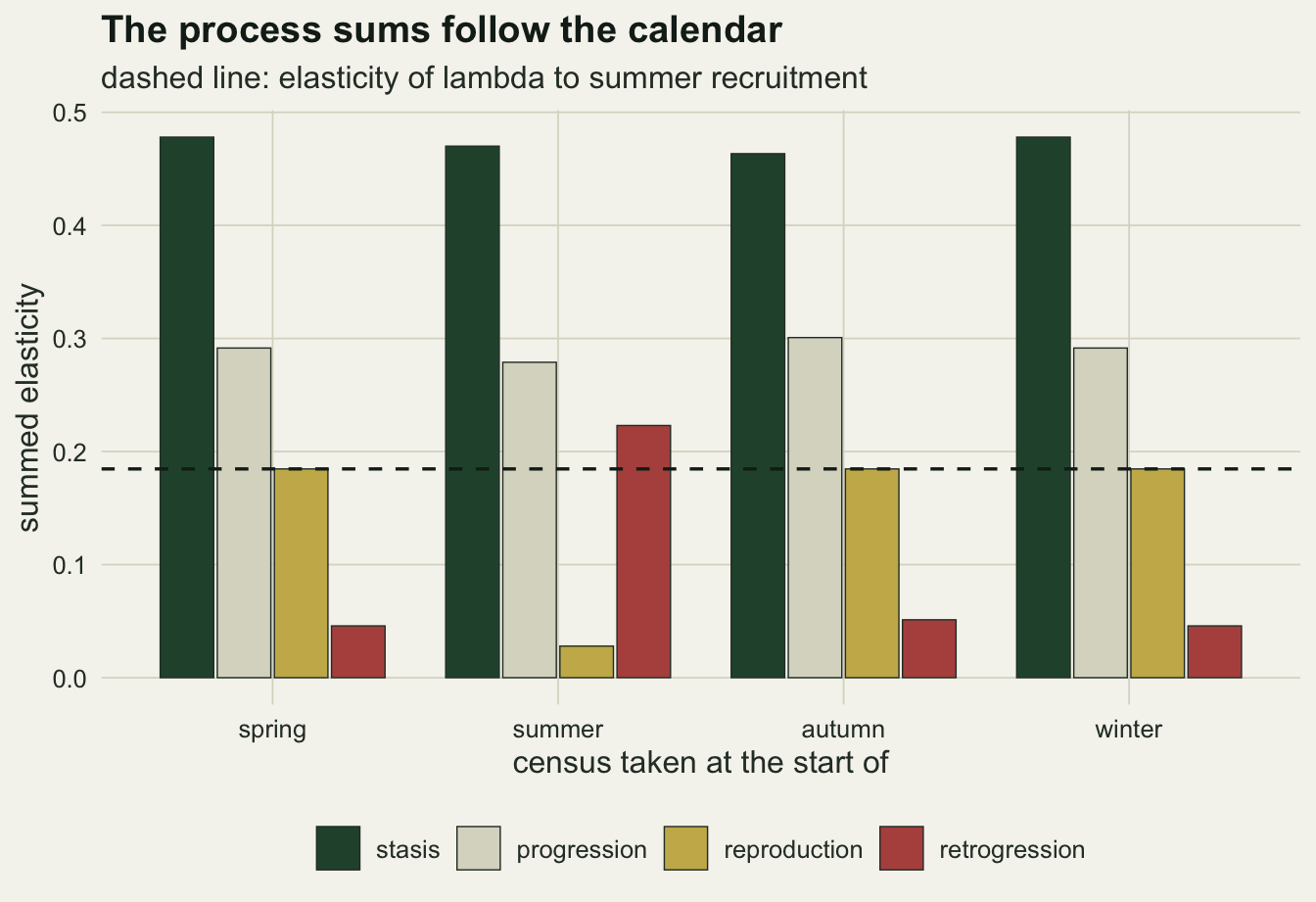
What to report
State the census date of every matrix, in the methods and next to every table of elasticities. Lambda can be compared across studies that censused at different times; stable stage distributions, reproductive values and elasticities of annual entries cannot.
If the seasonal transitions are known, publish the seasonal matrices, or the vital rates that build them, together with the order of multiplication. The annual matrix for any census date can be rebuilt from them and the reverse is not possible. Check the order with one eigenvalue: in this model the reversed product gave 1.1015 instead of 0.9806.
Base management rankings on elasticities to seasonal vital rates, computed with the periodic formula, and not on process sums of an annual matrix. When only an annual matrix exists, say which seasons each entry spans before giving it a process label; in this model 0.70 of the entry called retrogression at the midsummer census was recruitment followed by growth.
When comparing two annual matrices built at different dates, the similarity rule tells you whether any difference in elasticity could be an artefact: if the seasons between the two dates involve only survival, the elasticities agree exactly, and a difference between them cannot come from the census date.
Honest limits
The model is deterministic and has no sampling error. Real seasonal rates come from marked plants with binomial uncertainty, and a midsummer census may catch flowering plants better than an April one; detection that differs by census date would change the annual matrices as well, by an amount not measured here.
The change of headline entry at the midsummer census rests on a gap of 0.005 and is a property of these rates; other rates could give the same top entry at all four dates. The shift between reproduction and retrogression is the sturdier finding, because it follows from which seasons each annual entry spans rather than from the sizes of the rates, although its size is specific to this model.
Only survival and recruitment were analysed as vital rates. The movement probabilities enter the seasonal matrices as g in one cell and 1 - g in another, so their sensitivities are differences of entry sensitivities and can be negative; elasticities to them need the lower-level sensitivity step that Caswell described in 1978, and Caswell and Shyu extend the periodic case with matrix calculus. None of that changes the census independence, since it is still lambda as a function of seasonal rates.
The stage set here is the same at every census. If a stage is empty at some date, for instance if all seedlings become rosettes before a census, the seasonal matrices are rectangular and the products at different dates have different sizes. The nonzero eigenvalues are still shared, but the similarity rule no longer applies, and one of the square annual matrices may be reducible in the sense of Checking a matrix population model.
Finally, the seasons repeat exactly. Year to year variation in the seasonal rates turns lambda into a stochastic growth rate, and the stochastic growth rate of a random sequence of seasonal products needs its own treatment; census independence of the long-run rate still holds, but the elasticities are then averages over the sequence.
References
Caswell H, Trevisan MC 1994 Ecology 75(5):1299-1303 (10.2307/1937455)
Caswell H 1978 Theoretical Population Biology 14(2):215-230 (10.1016/0040-5809(78)90025-4)
de Kroon H, Plaisier A, van Groenendael J, Caswell H 1986 Ecology 67(5):1427-1431 (10.2307/1938700)
Caswell H, Shyu E 2012 Theoretical Population Biology 82(4):329-339 (10.1016/j.tpb.2012.03.008)
Caswell H 2001 Matrix Population Models, 2nd ed, Sinauer Associates (ISBN 978-0-87893-096-8)