---
title: "Pairwise PERMANOVA in R: which groups actually differ?"
description: "A significant PERMANOVA says your groups differ somewhere, not which pairs. Here is how to run post-hoc pairwise adonis2 in R, correct for multiple comparisons, and check dispersion before you trust the result."
date: "2026-06-21 14:00"
categories: [Multivariate, Hypothesis testing, vegan]
image: thumbnail.png
image-alt: "A grid of pairwise PERMANOVA p-values for four grazing levels, with significant cells shaded green."
---
You ran `adonis2()`, the p-value came back at 0.001, and the three stars look great in the output. Then a co-author asks the obvious question: *which* groups differ? A one-way PERMANOVA with four levels tests a single null hypothesis, that all four group centroids sit in the same place in multivariate space. Rejecting it tells you at least one group stands apart. It does not tell you whether every level differs from every other, or whether one odd group is carrying the whole result.
This post picks up where the [envfit and PERMANOVA tutorial](../envfit-and-permanova/) left off. There we tested whether grazing treatment explained community structure overall. Here we ask the follow-up that reviewers always want: a post-hoc breakdown of every pair, done honestly, with the multiple-testing problem handled and the dispersion assumption checked first.
## A grazing gradient where neighbours blur
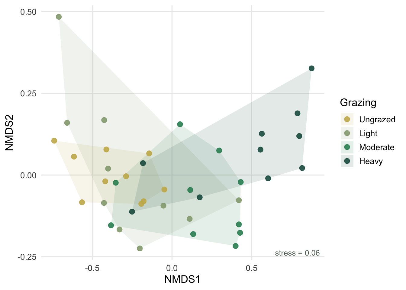
The teaching case is a grazing-intensity gradient with four levels: Ungrazed, Light, Moderate, and Heavy, ten plots each. Composition shifts gradually along the gradient, so adjacent levels overlap heavily while the extremes pull apart. That is exactly the situation where eyeballing an ordination misleads you and a formal pairwise test earns its keep.
```{r}
#| label: data
#| message: false
#| warning: false
library(vegan)
library(ggplot2)
library(dplyr)

set.seed(101)

groups   <- c("Ungrazed", "Light", "Moderate", "Heavy")
n_per    <- 10
grp      <- factor(rep(groups, each = n_per), levels = groups)

# latent gradient position per group, with within-group scatter so
# neighbouring levels overlap
g_center  <- c(Ungrazed = 0, Light = 0.6, Moderate = 1.2, Heavy = 1.8)
sd_within <- 0.70
latent    <- g_center[as.character(grp)] + rnorm(length(grp), 0, sd_within)

# 16 species with Gaussian niches spread across the gradient
n_sp  <- 16
opt   <- seq(-0.5, 2.3, length.out = n_sp)
width <- 1.0
peak  <- 18
lambda <- outer(latent, opt, function(x, o) peak * exp(-((x - o)^2) / (2 * width^2)))
comm   <- matrix(rpois(length(lambda), lambda), nrow = length(grp))
colnames(comm) <- paste0("sp", sprintf("%02d", seq_len(n_sp)))

dim(comm)
```
Forty plots, sixteen species, abundances drawn from Poisson noise around the niche model. The community is synthetic and illustrative; nothing here is a real survey.
## Step one: the omnibus test
Start with the test you already know. Compute Bray-Curtis distances and run the one-way PERMANOVA.
```{r}
#| label: omnibus
D <- vegdist(comm, method = "bray")

set.seed(42)
adonis2(D ~ grp, permutations = 999)
```
The model explains a little over 40% of the variation in Bray-Curtis distances and the permutation p-value lands at 0.001. Grazing matters. But four levels give six possible pairs, and this single number says nothing about how they sort out.
## Step two: check dispersion before you interpret
This step gets skipped constantly, and skipping it can invalidate everything that follows. PERMANOVA tests whether group centroids differ, but the permutation test is also sensitive to differences in *spread*. If one group is far more variable than another, you can get a significant result even when the centroids coincide. Anderson and Walsh (2013) walk through exactly how heterogeneous dispersion leaks into these tests.
So before any pairwise comparison, ask whether the groups are equally dispersed. `betadisper()` measures each plot's distance to its group centroid; `permutest()` tests whether those mean distances differ.
```{r}
#| label: dispersion
bd <- betadisper(D, grp)

set.seed(42)
permutest(bd, permutations = 999)
```
The dispersion test is non-significant (p well above 0.05), and the mean distance-to-centroid is similar across the four levels. That is the result you want here: with homogeneous dispersion, a significant PERMANOVA can be read as a genuine shift in composition rather than an artefact of one group being noisier. If this test *had* come back significant, you would need to report it and temper any location-based claim, because a "difference" might then be a difference in spread.
## Step three: pairwise comparisons
There is no `pairwise.adonis2()` in base vegan, but the logic is short to write yourself, which also keeps you honest about what it does. Loop over every pair of levels, subset the distance matrix to just those plots, and run `adonis2()` on the subset. Setting the seed before each call keeps the permutation p-values reproducible.
```{r}
#| label: pairwise
pairs <- combn(levels(grp), 2, simplify = FALSE)

res <- lapply(pairs, function(pr) {
  keep <- grp %in% pr
  Dsub <- as.dist(as.matrix(D)[keep, keep])
  set.seed(42)
  a <- adonis2(Dsub ~ grp[keep], permutations = 999)
  data.frame(
    group1 = pr[1], group2 = pr[2],
    R2 = round(a$R2[1], 3), F = round(a$F[1], 2),
    p_raw = a$`Pr(>F)`[1]
  )
})
pw <- do.call(rbind, res)
pw
```
Look at the raw p-values and a pattern jumps out. Every neighbouring pair (Ungrazed versus Light, Light versus Moderate, Moderate versus Heavy) is non-significant or borderline. Every pair two or more steps apart is strongly significant. The gradient is real, but its resolution is coarse: you cannot tell adjacent grazing levels apart from their plant communities, only the wider contrasts.
## Step four: correct for multiple comparisons
Six tests at a 0.05 threshold means roughly a one-in-four chance of at least one false positive if nothing were going on. You have to adjust. `p.adjust()` does both common corrections in one line each.
```{r}
#| label: correct
pw$p_bonf <- round(p.adjust(pw$p_raw, method = "bonferroni"), 3)
pw$p_BH   <- round(p.adjust(pw$p_raw, method = "BH"), 3)
pw
```
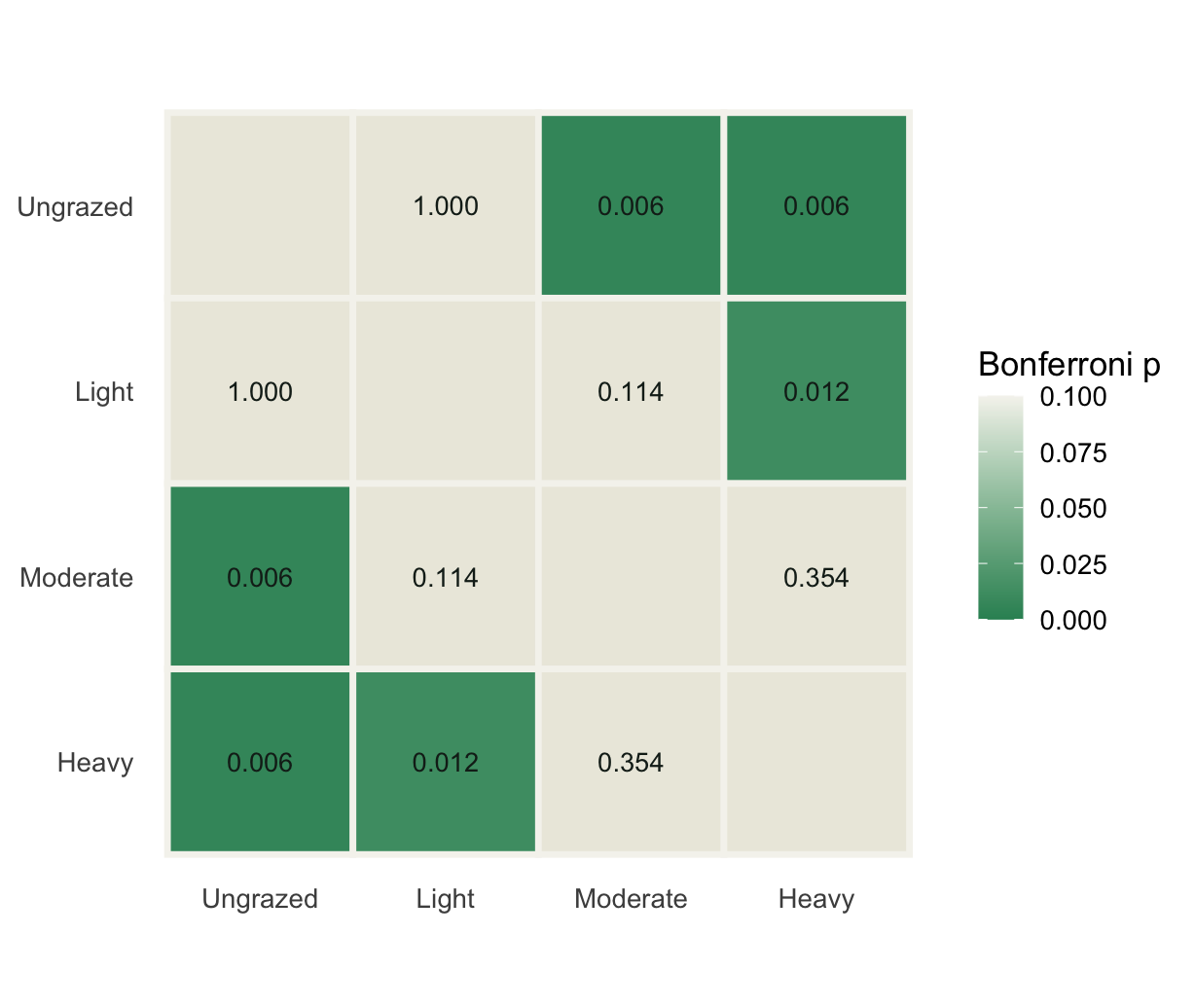
Two corrections, two philosophies. Bonferroni controls the family-wise error rate: the probability of even one false positive across all six tests. It is strict, and under it only the well-separated pairs survive. Benjamini and Hochberg (1995) instead control the false discovery rate, the expected proportion of false positives among the calls you make significant. It is more forgiving, and here it tips one borderline pair, Light versus Moderate, over the line that Bonferroni keeps it behind. Neither is "correct"; they answer different questions. The honest move is to pick one before you look at the results and report which you used, rather than choosing the threshold that gives the answer you wanted.
## Seeing the structure
Two figures make the story legible. An NMDS shows the overlap directly, and a tile grid shows which pairs cleared the bar.
```{r}
#| label: nmds
#| message: false
#| warning: false
#| fig-cap: "NMDS of the four grazing levels. Hulls mark within-group spread; neighbours overlap, extremes separate."
#| fig-width: 7
#| fig-height: 5
set.seed(7)
mds <- metaMDS(comm, distance = "bray", k = 2, trymax = 100,
               autotransform = FALSE, trace = FALSE)

scores_df <- as.data.frame(scores(mds, display = "sites"))
scores_df$grp <- grp

pal4 <- c(Ungrazed = "#c9b458", Light = "#93a87f",
          Moderate = "#2f8f63", Heavy = "#1d5b4e")
hulls <- scores_df %>% group_by(grp) %>% slice(chull(NMDS1, NMDS2))

ggplot(scores_df, aes(NMDS1, NMDS2, colour = grp, fill = grp)) +
  geom_polygon(data = hulls, alpha = 0.12, colour = NA) +
  geom_point(size = 2.6, alpha = 0.9) +
  scale_colour_manual(values = pal4, name = "Grazing") +
  scale_fill_manual(values = pal4, name = "Grazing") +
  annotate("text", x = Inf, y = -Inf,
           label = sprintf("stress = %.2f", mds$stress),
           hjust = 1.1, vjust = -0.8, size = 3.4, colour = "#5d6b61") +
  labs(x = "NMDS1", y = "NMDS2") +
  theme_minimal(base_size = 13) +
  theme(panel.grid.minor = element_blank())
```
```{r}
#| label: heatmap
#| fig-cap: "Pairwise PERMANOVA with Bonferroni-adjusted p-values. Green cells differ; blank cells are the same group."
#| fig-width: 6.4
#| fig-height: 5.4
mat <- expand.grid(g1 = levels(grp), g2 = levels(grp))
mat$p <- NA_real_
for (i in seq_len(nrow(pw))) {
  mat$p[mat$g1 == pw$group1[i] & mat$g2 == pw$group2[i]] <- pw$p_bonf[i]
  mat$p[mat$g2 == pw$group1[i] & mat$g1 == pw$group2[i]] <- pw$p_bonf[i]
}
mat$g1  <- factor(mat$g1, levels = levels(grp))
mat$g2  <- factor(mat$g2, levels = rev(levels(grp)))
mat$lab <- ifelse(is.na(mat$p), "",
                  ifelse(mat$p < 0.001, "<0.001",
                         formatC(mat$p, format = "f", digits = 3)))

ggplot(mat, aes(g1, g2, fill = p)) +
  geom_tile(colour = "#f5f4ee", linewidth = 1.2) +
  geom_text(aes(label = lab), size = 3.6, colour = "#16241d") +
  scale_fill_gradient(low = "#2f8f63", high = "#f5f4ee", na.value = "#eceadf",
                      name = "Bonferroni p", limits = c(0, 0.1)) +
  coord_equal() +
  labs(x = NULL, y = NULL) +
  theme_minimal(base_size = 13) +
  theme(panel.grid = element_blank())
```
## What to report
Write the omnibus result first, then the dispersion check, then the pairwise table with the correction named. A clean sentence for a methods section reads: a one-way PERMANOVA on Bray-Curtis distances found a significant effect of grazing (the figures here put it near 42% of variation, p = 0.001); dispersion was homogeneous (`betadisper`, p > 0.4), so the effect reflects composition rather than spread; pairwise PERMANOVA with Bonferroni correction separated levels two or more steps apart but not adjacent ones.
Three habits keep this defensible. Check dispersion before you interpret a location difference. Decide on your correction before you see the p-values. And remember that "non-significant" with ten plots per group means underpowered as easily as it means identical: a coarse gradient and a small sample look the same in this table. None of that is visible from the omnibus star rating, which is the whole reason to do the pairwise work.
## References
Anderson, M.J. (2001). A new method for non-parametric multivariate analysis of variance. *Austral Ecology*, 26(1), 32-46. https://doi.org/10.1111/j.1442-9993.2001.01070.pp.x
Anderson, M.J. & Walsh, D.C.I. (2013). PERMANOVA, ANOSIM, and the Mantel test in the face of heterogeneous dispersions: what null hypothesis are you testing? *Ecological Monographs*, 83(4), 557-574. https://doi.org/10.1890/12-2010.1
Benjamini, Y. & Hochberg, Y. (1995). Controlling the false discovery rate: a practical and powerful approach to multiple testing. *Journal of the Royal Statistical Society: Series B (Methodological)*, 57(1), 289-300. https://doi.org/10.1111/j.2517-6161.1995.tb02031.x