MCMC convergence diagnostics from scratch

Code the Gelman-Rubin R-hat and effective sample size by hand in R, and watch a single chain that looks perfectly converged miss half of a bimodal posterior.

A Markov chain sampler gives you draws, but it does not tell you whether those draws describe the posterior or only a corner of it. A chain can look completely settled, with a flat trace and a stable running mean, while sitting in one region it never leaves. The only way to catch that is to run several chains from different starting points and compare them numerically. This post codes the two standard checks by hand, the Gelman-Rubin statistic and the effective sample size, and uses a deliberately awkward target to show a single chain looking convincingly converged while missing half the answer.

A target built to trap a sampler

To make the point vividly we need a posterior with two well-separated peaks. A fifty-fifty mixture of two narrow normals, one at minus four and one at plus four, has a deep low-density valley between the modes. The same random-walk Metropolis sampler from the earlier posts will explore this, but with a small proposal it can sit in one mode almost forever, because crossing the valley requires a run of unlikely uphill-then-downhill moves.

log_post <- function(theta) log(0.5 * dnorm(theta, -4, 0.55) + 0.5 * dnorm(theta, 4, 0.55))

metropolis <- function(n_iter, prop_sd, init) {
  draws <- numeric(n_iter); cur <- init; cur_lp <- log_post(cur); acc <- 0L
  for (i in seq_len(n_iter)) {
    prop <- cur + rnorm(1, 0, prop_sd); prop_lp <- log_post(prop)
    if (log(runif(1)) < prop_lp - cur_lp) { cur <- prop; cur_lp <- prop_lp; acc <- acc + 1L }
    draws[i] <- cur
  }
  list(draws = draws, acc_rate = acc / n_iter)
}

# exact reference by a fine grid
gx <- seq(-8, 8, length.out = 200001)
gd <- 0.5 * dnorm(gx, -4, 0.55) + 0.5 * dnorm(gx, 4, 0.55)
gd <- gd / (sum(gd) * (gx[2] - gx[1]))
true_mean <- sum(gx * gd) * (gx[2] - gx[1])
true_q <- approx(cumsum(gd) * (gx[2] - gx[1]), gx, c(0.025, 0.975))$y
round(c(true_mean = true_mean, lower = true_q[1], upper = true_q[2]), 3)

true_mean     lower     upper 
    0.000    -4.905     4.905 

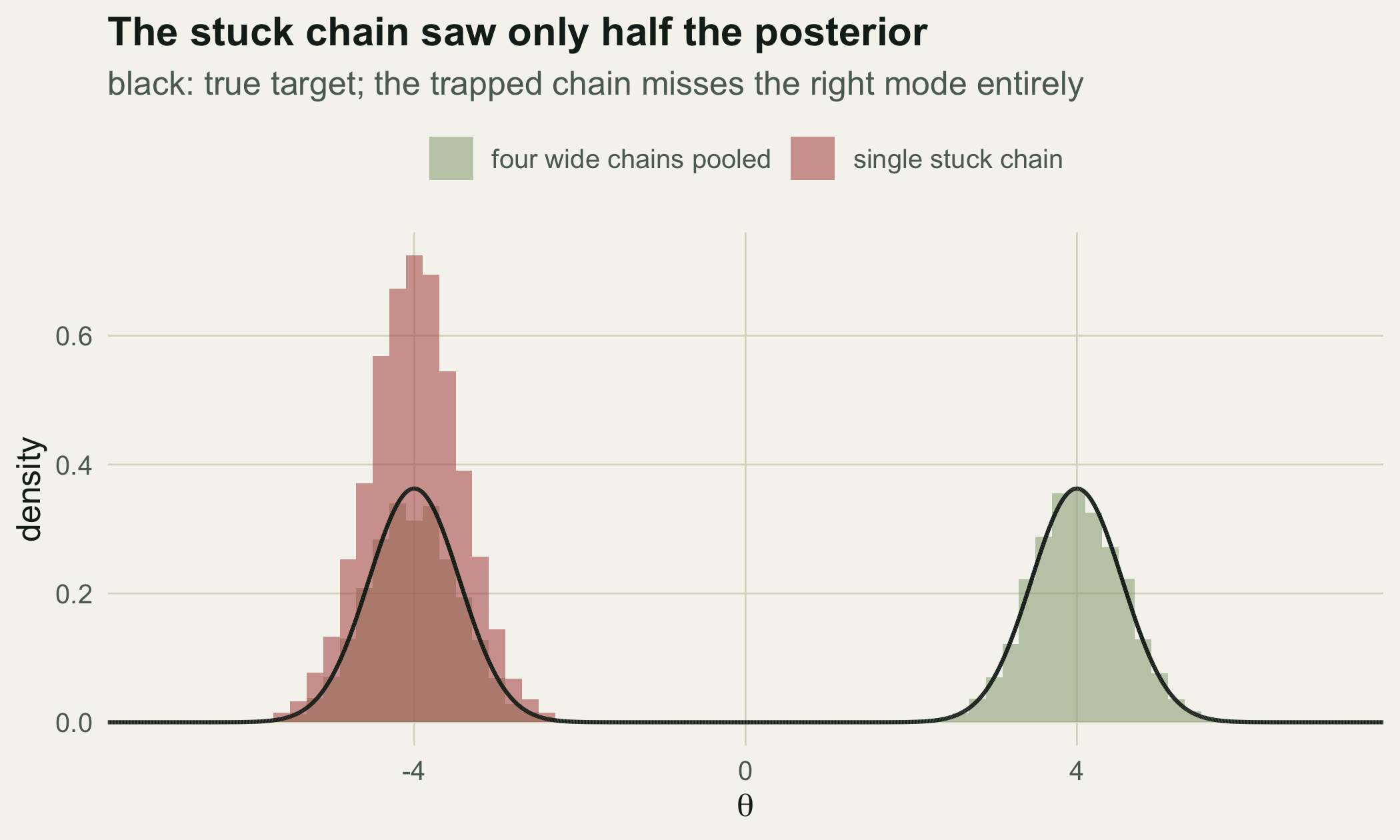
By symmetry the true posterior mean is 0 and the central 95 per cent of the mass runs from -4.9 to 4.9, spanning both modes. Any honest summary has to see both peaks.

A single chain that looks converged

Run one chain with a narrow proposal, started in the left mode, and summarise it. Drop the first 1500 iterations as burn-in.

n_iter <- 15000L; burn <- 1500L
keep <- (burn + 1):n_iter
set.seed(101)
solo <- metropolis(n_iter, prop_sd = 0.5, init = -4)$draws[keep]
round(c(mean = mean(solo), sd = sd(solo),
        lower = unname(quantile(solo, 0.025)), upper = unname(quantile(solo, 0.975))), 3)

  mean     sd  lower  upper 
-3.998  0.553 -5.106 -2.910 

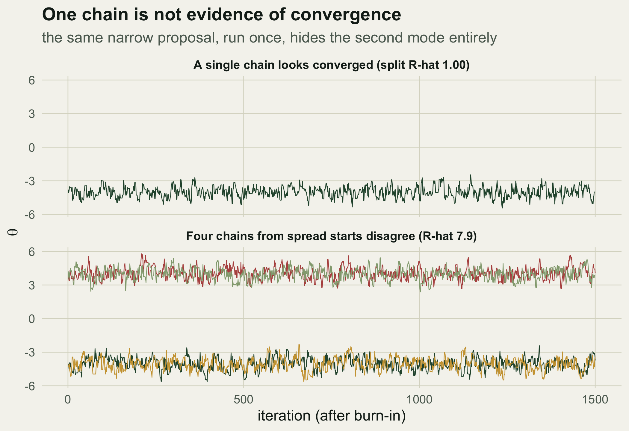
This chain looks flawless. Its running mean settles at -4, its trace is a stable band, and its 95 per cent interval is a tight -5.11 to -2.91. Every within-chain check passes. There is only one problem: the true posterior puts half its mass near plus four, and this chain never went there. Its interval misses the entire right mode. A single chain cannot know what it has not visited.

R-hat: comparing several chains

The Gelman-Rubin statistic formalises the idea of comparing chains. Run several from over-dispersed starts, then contrast the variance between the chain means with the variance within each chain. If the chains have converged to the same distribution, the two agree and the ratio is near one. If they sit in different places, the between-chain variance inflates the ratio. The split version cuts each chain in half first, so a single chain that drifts also gets caught.

rhat_split <- function(mat) {                 # mat: iterations x chains
  n <- nrow(mat); half <- n %/% 2
  sp <- cbind(mat[1:half, , drop = FALSE], mat[(n - half + 1):n, , drop = FALSE])
  n2 <- half
  cm <- colMeans(sp); cv <- apply(sp, 2, var)
  W <- mean(cv); B <- n2 * var(cm)             # within and between variance
  var_plus <- ((n2 - 1) / n2) * W + B / n2
  sqrt(var_plus / W)
}

The single chain alone passes even this test: its split R-hat is 1, because both halves sit in the same mode. Now run four chains from spread-out starts and compute R-hat across them.

starts <- c(-7, -3, 3, 7)
set.seed(202)
narrow <- sapply(starts, function(s) metropolis(n_iter, 0.5, s)$draws)
narrow_k <- narrow[keep, ]
rhat_narrow <- rhat_split(narrow_k)
round(c(chain_means = colMeans(narrow_k)), 2)

chain_means1 chain_means2 chain_means3 chain_means4 
       -4.03        -4.01         4.00         3.97 

The four chain means are split between the two modes, near minus four and near plus four, and R-hat jumps to 7.9. A value that far above one is a loud signal that the chains have not converged to a common distribution. The picture makes the contrast plain: one chain looks settled, four reveal the trap.

K <- 1500
chain_cols <- c("1" = forest, "2" = warm, "3" = brick, "4" = sage)
solo_df <- data.frame(iter = 1:K, value = solo[1:K], chain = "1",
                      panel = "A single chain looks converged (split R-hat 1.00)")
nar <- narrow_k[1:K, ]
narrow_df <- do.call(rbind, lapply(1:4, function(j)
  data.frame(iter = 1:K, value = nar[, j], chain = as.character(j),
             panel = "Four chains from spread starts disagree (R-hat 7.9)")))
tr <- rbind(solo_df, narrow_df)
tr$panel <- factor(tr$panel, levels = c("A single chain looks converged (split R-hat 1.00)",
                                        "Four chains from spread starts disagree (R-hat 7.9)"))
ggplot(tr, aes(iter, value, colour = chain)) +
  geom_line(linewidth = 0.3) +
  facet_wrap(~panel, ncol = 1) +
  scale_colour_manual(values = chain_cols, guide = "none") +
  labs(x = "iteration (after burn-in)", y = expression(theta),
       title = "One chain is not evidence of convergence",
       subtitle = "the same narrow proposal, run once, hides the second mode entirely")

Figure 1: Top: a single narrow-proposal chain, which looks converged and has split R-hat near one. Bottom: four chains from spread-out starts, which separate into two bands because each is stuck in a different mode.

Effective sample size

R-hat asks whether the chains agree. Effective sample size asks a different question: how many independent draws are these correlated samples worth? Successive Metropolis draws are autocorrelated, so a run of fifty thousand iterations carries far less information than fifty thousand independent draws. The estimate combines the autocorrelations across chains and sums them until the sequence turns negative.

ess_bda <- function(mat) {
  n <- nrow(mat); m <- ncol(mat)
  cm <- colMeans(mat); cv <- apply(mat, 2, var)
  W <- mean(cv); B <- n * var(cm)
  var_plus <- ((n - 1) / n) * W + B / n
  acov <- sapply(seq_len(m), function(j)
    acf(mat[, j], lag.max = n - 1, type = "covariance", plot = FALSE, demean = TRUE)$acf)
  acov_bar <- rowMeans(acov)                     # index 1 is lag 0
  rho <- 1 - (W - acov_bar[-1]) / var_plus         # combined autocorrelation
  tau <- 1; t <- 1                                 # Geyer initial positive sequence
  while (t + 1 <= length(rho)) {
    pair <- rho[t] + rho[t + 1]
    if (pair < 0) break
    tau <- tau + 2 * pair; t <- t + 2
  }
  (m * n) / tau
}
ess_narrow <- ess_bda(narrow_k)
round(c(stored_draws = length(narrow_k), effective = ess_narrow), 0)

stored_draws    effective 
       54000            2 

For the stuck chains the effective sample size is about 2 out of 54000 stored draws. That is not a rounding artefact: chains frozen in disagreement carry almost no usable information about the whole target, and the number says so. A high R-hat and a tiny effective sample size are two views of the same failure.

A sampler that actually mixes

The fix here is a proposal wide enough to jump the valley. With a large step the sampler occasionally proposes a move straight from one mode to the other and accepts it, so every chain visits both peaks.

set.seed(303)
wide <- sapply(starts, function(s) metropolis(n_iter, 4.0, s)$draws)
wide_k <- wide[keep, ]
rhat_wide <- rhat_split(wide_k)
ess_wide  <- ess_bda(wide_k)
round(c(rhat = rhat_wide, ess = ess_wide, pooled_mean = mean(wide_k),
        frac_left = mean(wide_k < 0)), 3)

       rhat         ess pooled_mean   frac_left 
      1.001    1346.452       0.096       0.487 

Now R-hat is 1.001, comfortably below the usual 1.01 threshold, and the effective sample size is about 1346. The pooled mean is 0.1, close to the true 0, and 49 per cent of the draws sit in the left mode, recovering the fifty-fifty split. The wide proposal pays for this with a lower acceptance rate, since many big steps land in the valley and are rejected, but that trade is worth it: a chain that accepts most of its moves yet never leaves one mode is worse than a choosier chain that explores the whole space. The recovered posterior shows both modes where the stuck chain showed one.

dens <- data.frame(x = gx, dens = gd)
hist_df <- rbind(
  data.frame(v = solo, src = "single stuck chain"),
  data.frame(v = as.vector(wide_k), src = "four wide chains pooled"))
hist_df$src <- factor(hist_df$src, levels = c("four wide chains pooled", "single stuck chain"))
ggplot() +
  geom_histogram(data = hist_df, aes(v, after_stat(density), fill = src),
                 binwidth = 0.2, colour = NA, alpha = 0.55, position = "identity") +
  geom_line(data = dens, aes(x, dens), colour = ink, linewidth = 0.7) +
  scale_fill_manual(values = c("four wide chains pooled" = sage, "single stuck chain" = brick), name = NULL) +
  coord_cartesian(xlim = c(-7, 7)) +
  labs(x = expression(theta), y = "density",
       title = "The stuck chain saw only half the posterior",
       subtitle = "black: true target; the trapped chain misses the right mode entirely")

Figure 2: The pooled draws from four wide chains (green) trace the true bimodal target (black), while the single stuck chain (red) covers only the left mode. Passing diagnostics correspond to seeing the whole posterior.

What to check, every time

This target was built to be hard, but the lesson is general. Run at least four chains from over-dispersed starting values. Compute split R-hat and require it below about 1.01 for every quantity you report, not just the mean. Check the effective sample size and make sure it is large enough for the precision you claim, typically a few hundred at least. Look at the trace and the autocorrelation as a sanity check, but do not rely on eyeballing a single chain, because a stuck chain and a converged chain can look identical. None of this proves a sampler is correct; it can only reveal problems. The next post puts these checks to work on a hierarchical model that mixes a Gibbs step with a Metropolis step, where several parameters have to converge together.

Related tutorials

• Metropolis-Hastings from scratch
• Gibbs sampling with conjugate updates
• Bayesian hierarchical models with MCMC
• Reproducible statistical workflow

References

• Gelman A, Rubin DB 1992 Statistical Science 7(4):457-472 (10.1214/ss/1177011136)
• Brooks SP, Gelman A 1998 Journal of Computational and Graphical Statistics 7(4):434-455 (10.1080/10618600.1998.10474787)
• Vehtari A, Gelman A, Simpson D, Carpenter B, Burkner PC 2021 Bayesian Analysis 16(2):667-718 (10.1214/20-BA1221)
• Geyer CJ 1992 Statistical Science 7(4):473-483 (10.1214/ss/1177011137)
• Gelman A, Carlin JB, Stern HS, Dunson DB, Vehtari A, Rubin DB 2013 Bayesian Data Analysis, 3rd edition (ISBN 978-1-4398-4095-5)