---
title: "Sensitivity and elasticity of matrix models"
description: "Compute sensitivity and elasticity of a population matrix in R, verify the eigenvector formula numerically, and rank vital rates for conservation action."
date: 2026-07-05 12:00
categories: [R, population dynamics, matrix models, conservation, ecology tutorial]
image: thumbnail.png
image-alt: "Heatmap of matrix elasticities with the largest value on the large-adult stasis entry"
---
Once you have a population matrix and its growth rate `lambda`, the practical question is which vital rate to act on. If you could raise adult survival, or seedling establishment, or fecundity, which change would move `lambda` the most? Sensitivity and elasticity answer this, and they are the reason matrix models are a conservation staple. This post computes both for the [stage matrix](../stage-structured-lefkovitch/) from the previous post, checks the analytical formula against brute-force perturbation, and shows why sensitivity and elasticity can point at different entries.
## Sensitivity: the slope of lambda
Sensitivity asks how much `lambda` changes for a small absolute change in a single matrix entry. There is a clean formula: the sensitivity of `lambda` to entry `a_ij` is the product of the reproductive value of stage `i` and the stable abundance of stage `j`, divided by their scalar product.
```{r}
#| label: setup
#| message: false
#| warning: false
library(ggplot2)
library(dplyr)
library(tidyr)

te_ink <- "#16241d"; te_forest <- "#275139"; te_mown <- "#2f8f63"
te_gold <- "#c9b458"; te_faint <- "#5d6b61"; te_line <- "#dad9ca"; te_paper <- "#f5f4ee"
theme_te <- function(base_size = 12) {
  theme_minimal(base_size = base_size) +
    theme(text = element_text(colour = "#2c3a31"),
          plot.title = element_text(colour = te_ink, face = "bold", size = base_size * 1.15),
          plot.subtitle = element_text(colour = te_faint, size = base_size * 0.95),
          axis.title = element_text(colour = "#46604a"), axis.text = element_text(colour = te_faint),
          panel.grid.minor = element_blank(),
          panel.grid.major = element_line(colour = te_line, linewidth = 0.3),
          plot.background = element_rect(fill = te_paper, colour = NA),
          panel.background = element_rect(fill = te_paper, colour = NA),
          legend.key = element_rect(fill = te_paper, colour = NA))
}

stages <- c("Seedling", "Juvenile", "Small adult", "Large adult")
A <- matrix(0, 4, 4, dimnames = list(stages, stages))
A["Juvenile",    "Seedling"]    <- 0.30
A["Juvenile",    "Juvenile"]    <- 0.35
A["Small adult", "Juvenile"]    <- 0.30
A["Small adult", "Small adult"] <- 0.45
A["Large adult", "Small adult"] <- 0.25
A["Seedling",    "Small adult"] <- 1.60
A["Large adult", "Large adult"] <- 0.82
A["Seedling",    "Large adult"] <- 3.00

ev  <- eigen(A)
lam <- Re(ev$values[1])
w   <- Re(ev$vectors[, 1]);        w <- w / sum(w)     # stable stage distribution
v   <- Re(eigen(t(A))$vectors[, 1]); v <- v / v[1]     # reproductive value
S   <- outer(v, w) / sum(v * w)                        # sensitivity matrix
dimnames(S) <- dimnames(A)
round(S, 3)
```
The largest entry in the sensitivity matrix is not one of the transitions the plant actually makes. It sits at the large-adult row and seedling column, an entry that is zero in the matrix because a seedling cannot become a large adult in a single year. Sensitivity does not care whether an entry is currently zero or biologically possible; it reports the slope as if that entry could take any value. That is a feature for evolutionary questions and a trap for management, which is where elasticity comes in.
Before trusting the formula, it is worth checking it the slow way: nudge each entry by a tiny amount, recompute `lambda`, and compare.
```{r}
#| label: numerical-check
delta <- 1e-6
S_num <- matrix(NA, 4, 4)
for (i in 1:4) for (j in 1:4) {
  Ap <- A; Ap[i, j] <- Ap[i, j] + delta
  S_num[i, j] <- (Re(eigen(Ap)$values[1]) - lam) / delta
}
max(abs(S - S_num))
```
The analytical sensitivities match the numerical ones to within a millionth, so the eigenvector formula is doing exactly what a brute-force perturbation would, at a fraction of the cost.
## Elasticity: proportional and comparable
Sensitivity mixes units. A survival probability lives between zero and one, while a fecundity can be several offspring, so their raw sensitivities are not comparable. Elasticity fixes this by scaling each sensitivity by the entry's own value relative to `lambda`. Elasticities are proportional sensitivities, they are dimensionless, they are zero wherever the matrix is zero, and they sum to one.
```{r}
#| label: elasticity
E <- (A / lam) * S
round(E, 3)
sum(E)
```
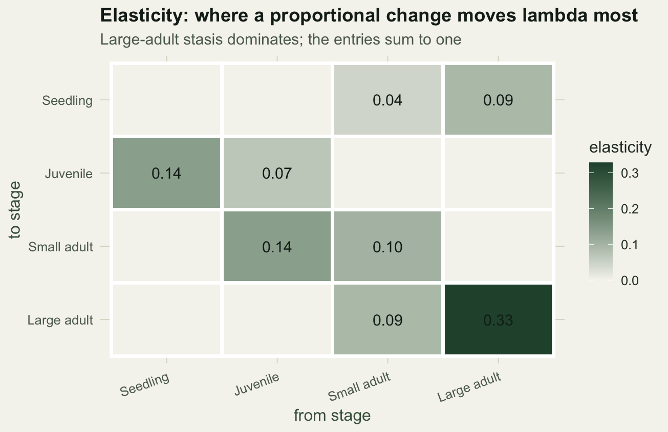
The elasticities sum to one, a result noted by de Kroon and colleagues, which lets you read each entry as a share of the total. The largest elasticity is the large-adult stasis term, the probability that a large adult survives and stays large. Unlike the sensitivity ranking, elasticity ignores the impossible seedling-to-large-adult jump, because that entry is zero.
```{r}
#| label: fig-elasticity
#| fig-cap: "Elasticity of each matrix entry; large-adult stasis carries the most weight."
#| fig-alt: "Heatmap of the four by four elasticity matrix; most cells are pale, the large-adult stasis cell on the diagonal is darkest at 0.33."
#| fig-width: 6.8
#| fig-height: 4.4
df <- as.data.frame(as.table(E)); colnames(df) <- c("to", "from", "elas")
df$to <- factor(df$to, levels = rev(stages)); df$from <- factor(df$from, levels = stages)
df$lab <- ifelse(df$elas > 0.0005, sprintf("%.2f", df$elas), "")
ggplot(df, aes(from, to, fill = elas)) +
  geom_tile(colour = "white", linewidth = 1.2) +
  geom_text(aes(label = lab), colour = te_ink, size = 4) +
  scale_fill_gradient(low = te_paper, high = te_forest, name = "elasticity") +
  labs(title = "Elasticity: where a proportional change moves lambda most",
       subtitle = "Large-adult stasis dominates; the entries sum to one",
       x = "from stage", y = "to stage") +
  theme_te() +
  theme(panel.grid = element_blank(), axis.text.x = element_text(angle = 20, hjust = 1))
```
## Which process matters for management
Because elasticities are comparable and additive, you can sum them by the kind of demographic process each entry represents: stasis, growth, or fecundity. That sum is the answer to the conservation question.
```{r}
#| label: by-process
proc <- matrix("", 4, 4)
for (i in 1:4) for (j in 1:4) {
  if (A[i, j] == 0) next
  if (i == 1 && j >= 3) proc[i, j] <- "Fecundity"
  else if (i == j)      proc[i, j] <- "Stasis"
  else                  proc[i, j] <- "Growth"
}
round(tapply(E[proc != ""], proc[proc != ""], sum), 3)
```
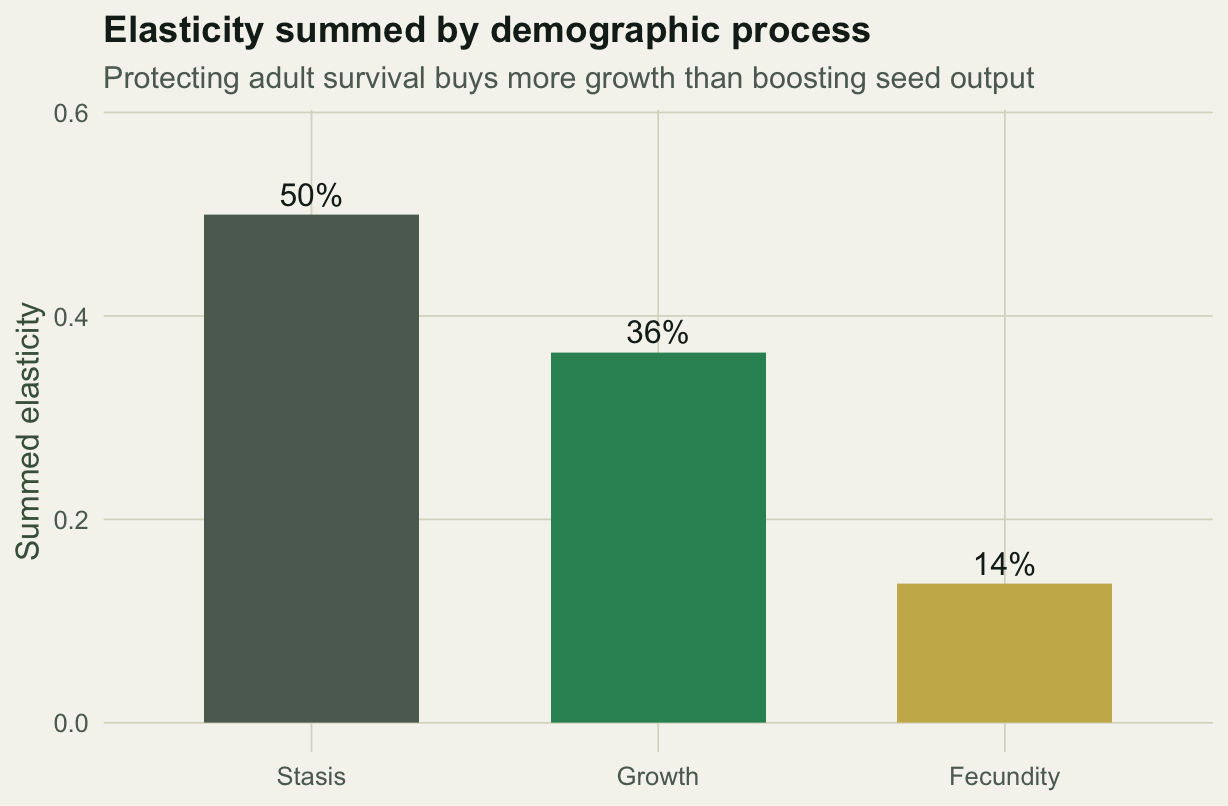
Half of the total elasticity is in stasis, mostly the persistence of large adults, and only about a seventh is in fecundity. For this population, a proportional gain in adult survival buys far more growth than the same proportional gain in seed output. That is the classic result for long-lived organisms, and it is exactly what Crouse and colleagues found for loggerhead sea turtles in 1987: management had focused on protecting eggs, the least responsive stage, when protecting large juveniles and adults would have done far more.
```{r}
#| label: fig-process
#| fig-cap: "Elasticity summed by process; adult survival dominates growth and fecundity."
#| fig-alt: "Bar chart of summed elasticity by demographic process: stasis about fifty percent, growth about thirty-six percent, fecundity about fourteen percent."
#| fig-width: 6.4
#| fig-height: 4.2
byproc <- tapply(E[proc != ""], proc[proc != ""], sum)
data.frame(process = factor(names(byproc), levels = c("Stasis", "Growth", "Fecundity")),
           elas = as.numeric(byproc)) |>
  ggplot(aes(process, elas)) +
  geom_col(aes(fill = process), width = 0.62, show.legend = FALSE) +
  geom_text(aes(label = sprintf("%.0f%%", 100 * elas)), vjust = -0.4, colour = te_ink, size = 4.2) +
  scale_fill_manual(values = c(Stasis = te_faint, Growth = te_mown, Fecundity = te_gold)) +
  ylim(0, max(byproc) * 1.15) +
  labs(title = "Elasticity summed by demographic process",
       subtitle = "Protecting adult survival buys more growth than boosting seed output",
       x = NULL, y = "Summed elasticity") +
  theme_te()
```
## What to take away
Sensitivity and elasticity turn a population matrix into a priority list. Sensitivity is the absolute slope of `lambda` against each entry, given exactly by reproductive value times stable abundance, and it will happily rank an entry that is biologically zero, which suits evolutionary questions but not management. Elasticity is the proportional version: dimensionless, comparable across survival and fecundity, summing to one, and zero where the matrix is zero. Summed by process it tells a manager where effort pays off, and for long-lived species that is usually adult survival, not fecundity. The formula matches brute-force perturbation to within rounding, so there is never a reason to compute it the slow way.
## References
- Caswell H 1978 Theoretical Population Biology 14(2):215-230 (10.1016/0040-5809(78)90025-4)
- de Kroon H, Plaisier A, van Groenendael J, Caswell H 1986 Ecology 67(5):1427-1431 (10.2307/1938700)
- Crouse DT, Crowder LB, Caswell H 1987 Ecology 68(5):1412-1423 (10.2307/1939225)
- Caswell H 2001 Matrix Population Models, 2nd ed, Sinauer Associates (ISBN 978-0-87893-096-8)
- Gotelli NJ 2008 A Primer of Ecology, 4th ed, Sinauer Associates (ISBN 978-0-87893-318-1)
## Related tutorials
- [Stage-structured Lefkovitch matrices in R](../stage-structured-lefkovitch/)
- [Leslie matrix population models in R](../leslie-matrix-population-models/)
- [Life tables and population growth in R](../life-tables-and-lambda/)