---
title: "Pseudoreplication and random intercepts: GLMMs for nested count data in R"
description: "Why nesting (plots within sites) breaks the independence assumption of a Poisson GLM, how a random intercept fixes it, and what intraclass correlation and partial pooling mean for ecological counts."
date: "2026-06-23 11:00"
categories: [R, Mixed models, GLMM, Count data, lme4]
image: thumbnail.png
image-alt: "Coefficient plot showing a plain GLM giving a far-too-narrow confidence interval for a site-level predictor compared with a mixed model."
---
Ecological count data rarely arrives as a flat list of independent observations. You count seedlings in several plots per site, across many sites; you revisit each transect a few times; you sample several leaves per tree. Observations that share a group resemble each other more than observations from different groups, and that breaks the independence assumption sitting underneath an ordinary [Poisson GLM](../glm-count-data-abundance/). Ignore it and you get pseudoreplication: standard errors that are too small and p-values that are too sure of themselves (Hurlbert 1984). The standard fix is a random intercept, fitted as a generalized linear mixed model with `lme4`.
## When observations share a group
We simulate a survey with a familiar structure: many sites, each holding an unequal number of plots. Two things drive the counts. `canopy` openness varies from plot to plot **within** a site. `elev` is a property of the site itself, so every plot in a site carries the same value. On top of these, each site has its own baseline abundance, drawn at random: that is the random intercept.
```{r}
#| label: setup
#| message: false
#| warning: false
library(lme4)
library(ggplot2)

pal_a <- "#b5534e"; pal_b <- "#2f8f63"; pal_lo <- "#c9b458"; pal_hi <- "#1d5b4e"
ink <- "#16241d"; gline <- "#dad9ca"
th <- theme_minimal(base_size = 12) +
  theme(panel.grid.minor = element_blank(),
        panel.grid.major = element_line(color = gline, linewidth = 0.3),
        plot.title = element_text(face = "bold", size = 11.5, color = ink),
        legend.position = "right")

set.seed(2024)
S  <- 24                                    # sites
Ps <- sample(3:15, S, replace = TRUE)       # unequal plots per site (3 to 15)
site <- factor(rep(seq_len(S), Ps))
N <- length(site)

a      <- rnorm(S, 0, 0.7)                   # site random intercept (log scale), sigma = 0.7
elev_s <- rnorm(S, 0, 1)                      # site-level predictor: one value per site
canopy <- rnorm(N, 0, 1)                      # plot-level predictor: varies within a site
elev   <- elev_s[as.integer(site)]
count  <- rpois(N, exp(0.3 + 1.2 * canopy + 0.5 * elev + a[as.integer(site)]))

d <- data.frame(count, canopy, elev, site)
c(N = N, sites = S, plots_min = min(Ps), plots_max = max(Ps), mean_count = round(mean(count), 1))
```
## The pooled GLM is overconfident
Fit the same fixed-effects structure two ways: a plain GLM that treats all `r N` plots as independent, and a GLMM that adds a random intercept for `site`.
```{r}
#| label: fit
#| message: false
#| warning: false
m_glm   <- glm(count ~ canopy + elev, family = poisson, data = d)
m_glmer <- glmer(count ~ canopy + elev + (1 | site), family = poisson, data = d)

cg <- summary(m_glm)$coefficients
ce <- summary(m_glmer)$coefficients
comp <- data.frame(
  predictor = c("canopy (plot-level)", "elev (site-level)"),
  glm_est   = round(cg[c("canopy","elev"), 1], 3),
  glm_se    = round(cg[c("canopy","elev"), 2], 3),
  glmer_est = round(ce[c("canopy","elev"), 1], 3),
  glmer_se  = round(ce[c("canopy","elev"), 2], 3),
  se_ratio  = round(ce[c("canopy","elev"), 2] / cg[c("canopy","elev"), 2], 1),
  row.names = NULL)
comp
```
```{r}
#| label: fig-coef
#| message: false
#| warning: false
#| fig-width: 9
#| fig-height: 3.2
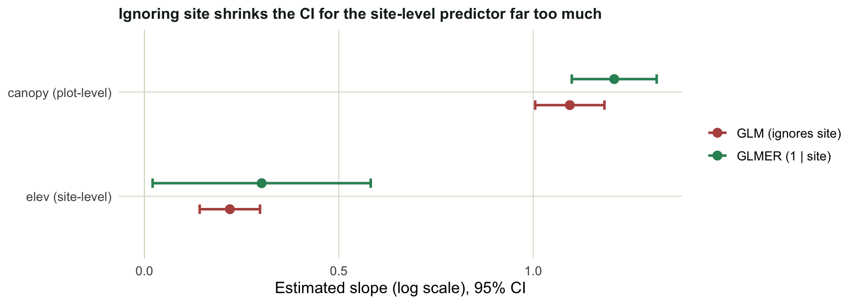
#| fig-cap: "Slope estimates with 95% confidence intervals. The two methods agree on the plot-level predictor; for the site-level predictor the plain GLM's interval is far too narrow."
ci <- function(co, meth) data.frame(term = c("canopy","elev"),
  est = co[c("canopy","elev"), 1], se = co[c("canopy","elev"), 2], method = meth)
cd <- rbind(ci(cg, "GLM (ignores site)"), ci(ce, "GLMER (1 | site)"))
cd$lo <- cd$est - 1.96 * cd$se; cd$hi <- cd$est + 1.96 * cd$se
cd$term <- factor(cd$term, levels = c("elev","canopy"),
                  labels = c("elev (site-level)","canopy (plot-level)"))

ggplot(cd, aes(est, term, color = method)) +
  geom_vline(xintercept = 0, color = gline, linewidth = 0.4) +
  geom_errorbarh(aes(xmin = lo, xmax = hi), height = 0.18, linewidth = 0.9,
                 position = position_dodge(0.5)) +
  geom_point(size = 2.8, position = position_dodge(0.5)) +
  scale_color_manual(values = c("GLM (ignores site)" = pal_a, "GLMER (1 | site)" = pal_b),
                     name = NULL) +
  labs(x = "Estimated slope (log scale), 95% CI", y = NULL,
       title = "Ignoring site shrinks the CI for the site-level predictor far too much") + th
```
The point estimates barely move. The uncertainty is where the methods part company. For `canopy`, which varies inside each site, the random intercept widens the standard error only slightly: a within-site comparison is already clean, because it is made against the site's own baseline. For `elev`, which is constant within a site, the standard error roughly triples. The plain GLM counts every plot as an independent piece of evidence about that site's `elev` value, so with eight plots per site it believes it has eight times the information it really has. That is pseudoreplication in one number: the GLM treats `elev` as overwhelmingly significant, while the honest mixed model, with a standard error more than three times larger, leaves the same effect only marginally significant.
## How much variation lives between sites
The random intercept is not just a correction; it is an estimate worth reading. Its variance tells you how much of the leftover variation is between sites rather than within them.
```{r}
#| label: icc
#| message: false
#| warning: false
vc   <- as.data.frame(VarCorr(m_glmer))
sig2 <- vc$vcov[vc$grp == "site"]
icc  <- sig2 / (sig2 + log(1 + 1 / mean(count)))     # latent-scale ICC (Nakagawa)
disp <- sum(residuals(m_glmer, "pearson")^2) / df.residual(m_glmer)
c(sigma_site = round(sqrt(sig2), 3),
  icc        = round(icc, 3),
  dispersion = round(disp, 2))
```
The between-site standard deviation lands near 0.59 on the log scale, so typical sites differ in baseline abundance by roughly `exp(0.59)`, about 1.8-fold. The intraclass correlation, here computed on the latent scale (Nakagawa, Johnson and Schielzeth 2017), is around 0.52, meaning about half the residual variation is between sites. That is a strong grouping, and exactly the situation where pretending the plots are independent does the most damage. The Pearson dispersion sits near 0.8, comfortably below 1, so a Poisson GLMM is adequate here and there is no need to move to a negative-binomial or observation-level random effect (the [count GLM post](../glm-count-data-abundance/) covers that path).
## Partial pooling and shrinkage
A mixed model does not estimate each site in isolation, and it does not lump them all together either. It does something in between, called partial pooling: each site's estimate is pulled toward the overall mean, and sites with less data are pulled harder, because their own counts are less trustworthy.
```{r}
#| label: fig-shrinkage
#| message: false
#| warning: false
#| fig-width: 6.6
#| fig-height: 4.2
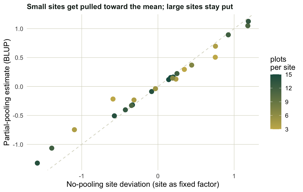
#| fig-cap: "Each site's deviation estimated two ways. No pooling fits every site separately; partial pooling (the BLUP) pulls estimates toward 0, and small sites move most."
m_sh <- glmer(count ~ canopy + (1 | site), family = poisson, data = d)
blup <- ranef(m_sh)$site[, 1]
m_np <- glm(count ~ canopy + factor(site) - 1, family = poisson, data = d)
sc   <- coef(m_np)[grep("factor", names(coef(m_np)))]
np_dev <- sc - mean(sc)
gs <- as.integer(table(site))
sh <- data.frame(np_dev, blup, gs)

ggplot(sh, aes(np_dev, blup, color = gs)) +
  geom_abline(slope = 1, intercept = 0, color = gline, linewidth = 0.5, linetype = 2) +
  geom_hline(yintercept = 0, color = gline, linewidth = 0.3) +
  geom_point(size = 3) +
  scale_color_gradient(low = pal_lo, high = pal_hi, name = "plots\nper site") +
  labs(x = "No-pooling site deviation (site as fixed factor)",
       y = "Partial-pooling estimate (BLUP)",
       title = "Small sites get pulled toward the mean; large sites stay put") + th
```
Points on the dashed line would mean no shrinkage at all. Instead the pale points, the sites with only three or four plots, sit well inside the line, dragged toward 0, while the dark points with a dozen plots or more hold their ground. This is partial pooling borrowing strength across the survey: a site with three noisy plots is told to look a little more like everyone else, which usually improves the prediction for that site.
## The cost of ignoring it: a type-I check
The clearest way to feel the danger is to simulate a true null and see how often each method cries wolf. We generate grouped data where a site-level predictor has no effect at all, fit both models, and record the p-value for that predictor. Over many repeats, a well-behaved test should reject at the nominal rate of 0.05.
```{r}
#| label: typeI
#| message: false
#| warning: false
sim1 <- function(seed) {
  set.seed(seed)
  S <- 15; P <- 8; site <- factor(rep(1:S, each = P)); N <- S * P
  a <- rnorm(S, 0, 0.7); z <- rnorm(S)[as.integer(site)]   # null site-level predictor
  y <- rpois(N, exp(0.4 + a[as.integer(site)]))            # z has no effect
  dd <- data.frame(y, z, site)
  pg <- tryCatch(summary(glm(y ~ z, family = poisson, data = dd))$coefficients["z", 4],
                 error = function(e) NA)
  pm <- tryCatch(suppressWarnings(suppressMessages(
        summary(glmer(y ~ z + (1 | site), data = dd, family = poisson))$coefficients["z", 4])),
        error = function(e) NA)
  c(glm = pg, glmer = pm)
}
R <- 300
ps <- as.data.frame(t(vapply(1:R, sim1, numeric(2))))
c(GLM_false_positive = round(mean(ps$glm   < 0.05, na.rm = TRUE), 3),
  GLMER_false_positive = round(mean(ps$glmer < 0.05, na.rm = TRUE), 3))
```
```{r}
#| label: fig-typeI
#| message: false
#| warning: false
#| fig-width: 9
#| fig-height: 3.4
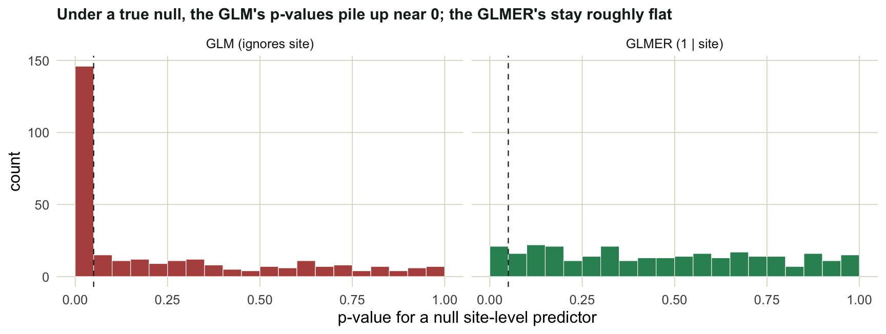
#| fig-cap: "Distribution of p-values for a predictor that genuinely does nothing. A calibrated test gives a flat histogram; the GLM is anything but."
pl <- rbind(data.frame(p = ps$glm,   method = "GLM (ignores site)"),
            data.frame(p = ps$glmer, method = "GLMER (1 | site)"))
ggplot(pl, aes(p, fill = method)) +
  geom_histogram(breaks = seq(0, 1, 0.05), color = "white", linewidth = 0.2) +
  geom_vline(xintercept = 0.05, color = ink, linetype = 2, linewidth = 0.4) +
  scale_fill_manual(values = c("GLM (ignores site)" = pal_a, "GLMER (1 | site)" = pal_b),
                    guide = "none") +
  facet_wrap(~method) +
  labs(x = "p-value for a null site-level predictor", y = "count",
       title = "Under a true null, the GLM's p-values pile up near 0; the GLMER's stay roughly flat") + th
```
The plain GLM rejects the null around 49% of the time, nearly ten times the rate it should, and its p-values heap up against 0. The mixed model lands near 0.07, close to the target, with a roughly flat histogram. The small overshoot is honest: Wald tests for mixed models run slightly liberal when the number of groups is modest, as it is here with 15 sites. The fix is the same family of remedy as in the [spatial autocorrelation post](../spatial-autocorrelation-morans-i/): when observations are not independent, model the dependence rather than assuming it away.
## Practical notes
Treat a factor as **random** when its levels are an exchangeable sample from a larger population you want to generalize to (sites, individuals, blocks) and there are enough of them, say five or more, to estimate a variance. Treat it as **fixed** when the levels are few and specifically of interest (two treatments, three years you care about by name). Always check dispersion after fitting; if the Pearson statistic runs well above 1, move to a negative-binomial GLMM or add an observation-level random effect (Harrison et al. 2018). Lean on the variance components and the ICC to describe your design, not just to pass a test. And remember that the Wald p-values printed by `summary` are approximate: for a result near the line, prefer a likelihood-ratio test or a profile or bootstrap confidence interval, and read the modelling guidance in Bolker et al. (2009).
## References
Bates, D., Maechler, M., Bolker, B. and Walker, S. (2015). Fitting linear mixed-effects models using lme4. *Journal of Statistical Software* 67(1): 1-48. <https://doi.org/10.18637/jss.v067.i01>
Hurlbert, S. H. (1984). Pseudoreplication and the design of ecological field experiments. *Ecological Monographs* 54(2): 187-211. <https://doi.org/10.2307/1942661>
Bolker, B. M., Brooks, M. E., Clark, C. J., Geange, S. W., Poulsen, J. R., Stevens, M. H. H. and White, J.-S. S. (2009). Generalized linear mixed models: a practical guide for ecology and evolution. *Trends in Ecology and Evolution* 24(3): 127-135. <https://doi.org/10.1016/j.tree.2008.10.008>
Harrison, X. A., Donaldson, L., Correa-Cano, M. E., Evans, J., Fisher, D. N., Goodwin, C. E. D., Robinson, B. S., Hodgson, D. J. and Inger, R. (2018). A brief introduction to mixed effects modelling and multi-model inference in ecology. *PeerJ* 6: e4794. <https://doi.org/10.7717/peerj.4794>
Nakagawa, S., Johnson, P. C. D. and Schielzeth, H. (2017). The coefficient of determination R2 and intra-class correlation coefficient from generalized linear mixed-effects models revisited and expanded. *Journal of the Royal Society Interface* 14(134): 20170213. <https://doi.org/10.1098/rsif.2017.0213>