---
title: "Gibbs sampling with conjugate updates"
description: "Build a Gibbs sampler in base R for the mean and variance of a trait, and see why the mean's posterior is a t distribution rather than a narrow normal."
date: "2026-07-14 10:00"
categories: [Bayesian statistics, MCMC, R, ecology tutorial]
image: thumbnail.png
image-alt: "A scatter of joint posterior draws for a mean and standard deviation, overlaid with a staircase path showing Gibbs updating one coordinate at a time."
---
The random-walk Metropolis sampler in the companion post has one fiddly part: a proposal width you have to tune, and a stream of rejected moves you have to accept as waste. When a model has a helpful structure, you can avoid both. If each parameter, holding the others fixed, has a posterior that is itself a standard distribution, you can draw from those one at a time and never reject anything. That is Gibbs sampling. This post codes it in base R for the simplest two-parameter problem an ecologist meets constantly: estimating the mean and the variance of a measured trait. Along the way it shows a mistake that is easy to make, treating the variance as if it were known once you have estimated it, which quietly shrinks the interval on the mean.
```{r}
#| label: setup
#| include: false
library(ggplot2)
knitr::opts_chunk$set(echo = TRUE, message = FALSE, warning = FALSE,
fig.align = "center", dpi = 150)
paper <- "#f5f4ee"; ink <- "#16241d"; forest <- "#275139"; sage <- "#93a87f"
line_col <- "#dad9ca"; faint <- "#5d6b61"; accent2 <- "#c9b458"; warm <- "#cda23f"; brick <- "#b5534e"
theme_te <- function(base = 12) theme_minimal(base_size = base) + theme(
plot.background = element_rect(fill = paper, colour = NA),
panel.background = element_rect(fill = paper, colour = NA),
panel.grid.major = element_line(colour = line_col, linewidth = 0.3),
panel.grid.minor = element_blank(),
axis.title = element_text(colour = ink), axis.text = element_text(colour = faint),
plot.title = element_text(colour = ink, face = "bold"),
plot.subtitle = element_text(colour = faint),
legend.title = element_text(colour = ink), legend.text = element_text(colour = faint),
legend.position = "top",
strip.text = element_text(colour = ink, face = "bold"))
theme_set(theme_te())
```
## The data and the two quantities
A dozen individuals of a hard-to-catch passerine are measured for wing length in millimetres. We want the population mean and also the population variance, because among-individual spread is itself an ecological quantity (it feeds selection gradients, size-based models, and detection).
```{r}
#| label: data
set.seed(2718)
n <- 12L
y <- rnorm(n, mean = 76, sd = 3.2)      # a small synthetic sample, wing length (mm)
ybar <- mean(y)
s2 <- var(y)                             # sample variance (denominator n - 1)
s  <- sqrt(s2)
round(c(n = n, ybar = ybar, s = s, s2 = s2), 3)
```
The sample mean is `r round(ybar, 2)` mm and the sample standard deviation is `r round(s, 2)` mm. With only `r n` birds, neither quantity is pinned down, and the uncertainty in the variance should leak into the uncertainty in the mean.
## The model and its full conditionals
Take the data as normal with unknown mean and variance, and use the standard reference prior $p(\mu, \sigma^2) \propto 1/\sigma^2$, which is flat on $\mu$ and on $\log \sigma$. The joint posterior has no simple one-line form, but each parameter conditional on the other does. Completing the square in $\mu$ and collecting powers of $\sigma^2$ gives two familiar distributions:
$$\mu \mid \sigma^2, y \;\sim\; \text{Normal}\!\left(\bar y,\; \sigma^2/n\right), \qquad \sigma^2 \mid \mu, y \;\sim\; \text{Inv-Gamma}\!\left(\tfrac{n}{2},\; \tfrac{1}{2}\textstyle\sum_i (y_i - \mu)^2\right).$$
Both are things we can sample directly. A normal draw is `rnorm`; an inverse-gamma draw is the reciprocal of a gamma draw, since if $X \sim \text{Gamma}(a, \text{rate}=b)$ then $1/X \sim \text{Inv-Gamma}(a, b)$. Gibbs simply alternates: draw a new mean given the current variance, then a new variance given the new mean, and repeat.
```{r}
#| label: sampler
gibbs <- function(n_iter, y, init_sigma2 = 1) {
  n <- length(y); ybar <- mean(y)
  mu <- numeric(n_iter); sig2 <- numeric(n_iter)
  cur_sig2 <- init_sigma2
  for (t in seq_len(n_iter)) {
    cur_mu   <- rnorm(1, ybar, sqrt(cur_sig2 / n))                 # mu | sigma^2, y
    ss       <- sum((y - cur_mu)^2)
    cur_sig2 <- 1 / rgamma(1, shape = n / 2, rate = ss / 2)        # sigma^2 | mu, y
    mu[t] <- cur_mu; sig2[t] <- cur_sig2
  }
  data.frame(mu = mu, sigma2 = sig2)
}
```
There is no proposal width, no accept step, and no rejected draw. The price is that every conditional had to be a distribution we can sample from, which here it is.
## Running the sampler
```{r}
#| label: run
n_iter <- 40000L; burn <- 2000L
set.seed(90210)
chain <- gibbs(n_iter, y, init_sigma2 = 1)
post  <- chain[(burn + 1):n_iter, ]
round(c(acf1_mu = acf(post$mu, 1, plot = FALSE)$acf[2],
        acf1_sigma2 = acf(post$sigma2, 1, plot = FALSE)$acf[2]), 3)
```
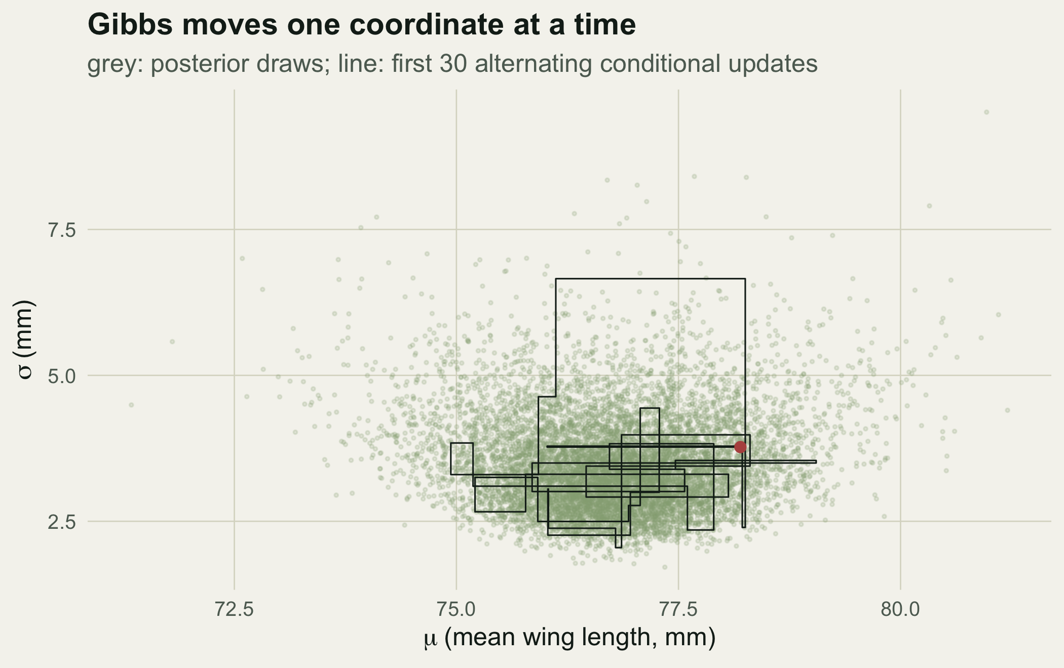
The lag-one autocorrelation is `r round(acf(post$mu,1,plot=FALSE)$acf[2], 3)` for the mean and `r round(acf(post$sigma2,1,plot=FALSE)$acf[2], 3)` for the variance: successive draws are practically independent, so the chain mixes far better than a tuned random walk would on the same target. The figure below shows how Gibbs gets there. It updates one coordinate at a time, so its path through the joint space is a staircase of horizontal and vertical moves rather than a diagonal drift.
```{r}
#| label: fig-staircase
#| fig-cap: "Joint posterior of the mean and standard deviation (grey draws) with the first 30 Gibbs iterations traced as a staircase. Each step moves the mean given the current variance, then the variance given the new mean."
#| fig-alt: "A grey cloud of joint posterior points for the mean and standard deviation, crossed by a black staircase path of alternating horizontal and vertical segments starting at a red dot."
#| fig-width: 7
#| fig-height: 4.4
sig <- sqrt(post$sigma2)
K <- 30
mu <- post$mu[1:K]; sg <- sig[1:K]
vx <- mu[1]; vy <- sg[1]
for (t in 2:K) { vx <- c(vx, mu[t], mu[t]); vy <- c(vy, sg[t-1], sg[t]) }
stair <- data.frame(x = vx, y = vy)
cloud <- data.frame(mu = post$mu, sigma = sig)[seq(1, nrow(post), by = 4), ]
ggplot() +
  geom_point(data = cloud, aes(mu, sigma), colour = sage, alpha = 0.20, size = 0.5) +
  geom_path(data = stair, aes(x, y), colour = ink, linewidth = 0.35) +
  geom_point(data = stair[1, ], aes(x, y), colour = brick, size = 2) +
  labs(x = expression(mu ~ "(mean wing length, mm)"), y = expression(sigma ~ "(mm)"),
       title = "Gibbs moves one coordinate at a time",
       subtitle = "grey: posterior draws; line: first 30 alternating conditional updates")
```
## Checking against the exact answer, and the naive shortcut
This model has a closed-form marginal for the mean. Under the reference prior, integrating the variance out of the joint posterior leaves a Student-t: $\mu \mid y \sim t_{n-1}(\bar y,\; s^2/n)$, the same t that underlies the one-sample confidence interval. That gives an exact target for the sampler and a clean contrast with the shortcut.
```{r}
#| label: marginals
mu_ci_gibbs <- quantile(post$mu, c(0.025, 0.975))
mu_ci_exact <- ybar + c(-1, 1) * qt(0.975, df = n - 1) * s / sqrt(n)   # exact t interval
mu_ci_naive <- ybar + c(-1, 1) * 1.96 * s / sqrt(n)                    # fix sigma at s, use normal
s2_ci_gibbs <- quantile(post$sigma2, c(0.025, 0.975))
s2_ci_exact <- (n - 1) * s2 / qchisq(c(0.975, 0.025), df = n - 1)      # exact for the variance
rbind(mu_gibbs = mu_ci_gibbs, mu_exact_t = mu_ci_exact, mu_naive = mu_ci_naive)
```
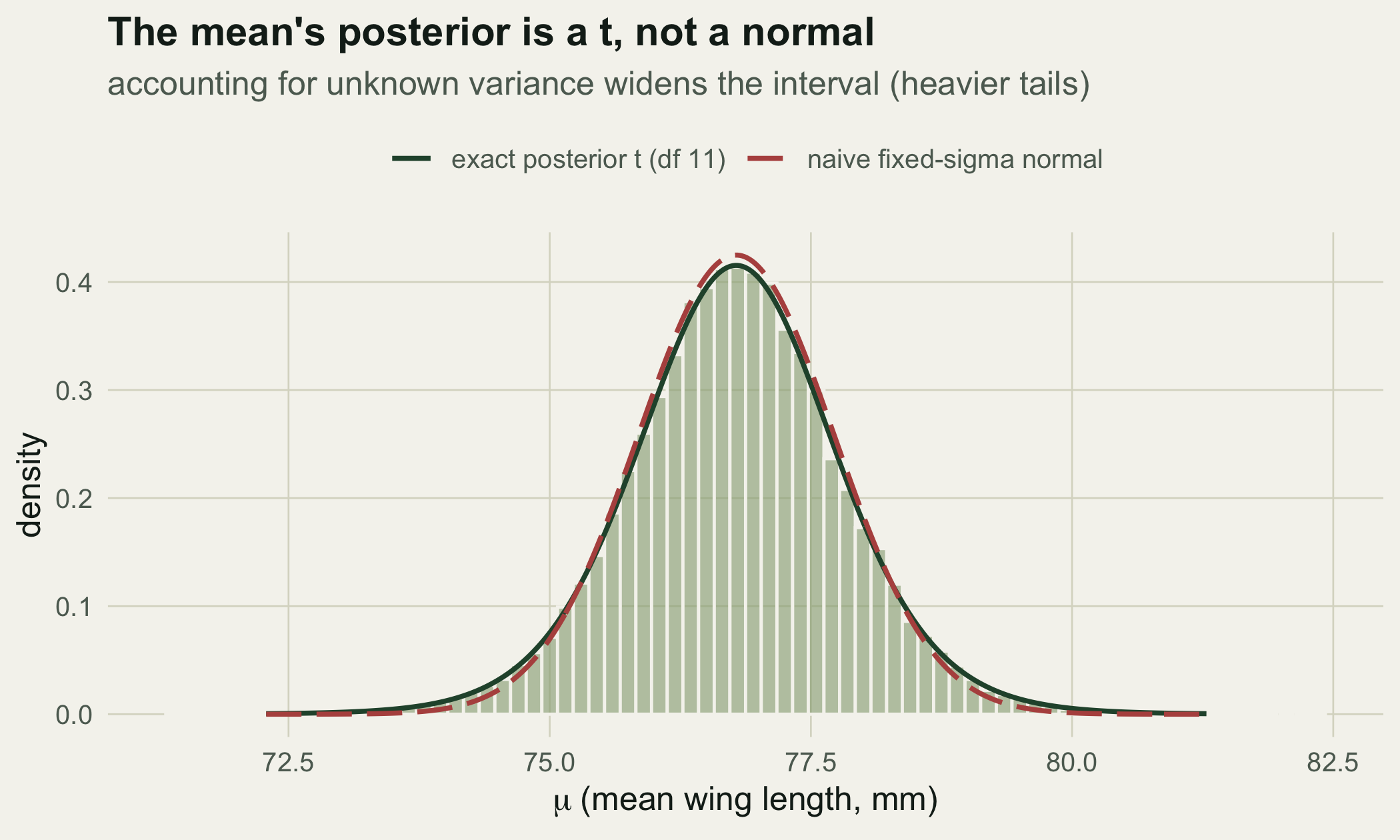
The Gibbs interval for the mean, `r round(mu_ci_gibbs[1], 2)` to `r round(mu_ci_gibbs[2], 2)`, lands on the exact t interval, `r round(mu_ci_exact[1], 2)` to `r round(mu_ci_exact[2], 2)`. The variance interval matches too: Gibbs gives `r round(s2_ci_gibbs[1], 2)` to `r round(s2_ci_gibbs[2], 2)` against the exact `r round(s2_ci_exact[1], 2)` to `r round(s2_ci_exact[2], 2)`. The naive interval, which fixes the standard deviation at its sample value and then treats the mean as normal, runs `r round(mu_ci_naive[1], 2)` to `r round(mu_ci_naive[2], 2)`. It is narrower, by `r round((diff(mu_ci_exact)/diff(mu_ci_naive) - 1) * 100, 1)` per cent here, and the gap grows as the sample shrinks. The next figure shows why: the mean's true posterior has the heavier tails of a t, and pretending the variance is known throws those tails away.
```{r}
#| label: fig-marginal
#| fig-cap: "Marginal posterior of the mean (bars) with the exact t density (solid) and the naive fixed-variance normal (dashed). The t is wider; ignoring uncertainty in the variance understates uncertainty in the mean."
#| fig-alt: "A histogram of mean draws overlaid with a solid forest t curve and a dashed red normal curve that is slightly taller and narrower."
#| fig-width: 7
#| fig-height: 4.2
xs <- seq(ybar - 4.5, ybar + 4.5, length.out = 400)
sc <- s / sqrt(n)
curv <- rbind(
  data.frame(x = xs, dens = dt((xs - ybar) / sc, df = n - 1) / sc, src = "exact posterior t (df 11)"),
  data.frame(x = xs, dens = dnorm(xs, ybar, sc), src = "naive fixed-sigma normal"))
curv$src <- factor(curv$src, levels = c("exact posterior t (df 11)", "naive fixed-sigma normal"))
ggplot() +
  geom_histogram(data = data.frame(mu = post$mu), aes(mu, after_stat(density)),
                 binwidth = 0.15, fill = sage, colour = paper, alpha = 0.6) +
  geom_line(data = curv, aes(x, dens, colour = src, linetype = src), linewidth = 0.85) +
  scale_colour_manual(values = c(forest, brick), name = NULL) +
  scale_linetype_manual(values = c("solid", "longdash"), name = NULL) +
  labs(x = expression(mu ~ "(mean wing length, mm)"), y = "density",
       title = "The mean's posterior is a t, not a normal",
       subtitle = "accounting for unknown variance widens the interval (heavier tails)")
```
## Gibbs or Metropolis
The joint draws also answer questions no single interval can. If a downstream model needs both a large mean and a wide spread, the posterior gives the joint probability straight from the stored columns: here about `r round(mean(post$mu > 77 & sqrt(post$sigma2) > 3.5) * 100)` per cent of draws have a mean above 77 mm and a standard deviation above 3.5 mm.
Gibbs and Metropolis are not rivals so much as tools for different situations. Gibbs needs conjugate conditionals but then runs with no tuning and little autocorrelation, which is why it dominates this normal model. When a conditional is not a standard distribution, you can still take a Metropolis step for that one parameter inside an otherwise-Gibbs loop, which is the pattern the hierarchical model in this series uses for its non-conjugate pieces. Either way, an independent check on convergence is still needed: a chain that looks settled in one run is not proof, and the diagnostics post shows how to test it with several chains and a numerical statistic.
## Related tutorials
- [Metropolis-Hastings from scratch](../metropolis-hastings-from-scratch/)
- [MCMC convergence diagnostics from scratch](../mcmc-convergence-diagnostics/)
- [Linear models: t-test and ANOVA in R](../linear-models-t-test-anova/)
- [Standard errors and confidence intervals](../standard-errors-confidence-intervals/)
## References
- Geman S, Geman D 1984 IEEE Transactions on Pattern Analysis and Machine Intelligence 6(6):721-741 (10.1109/TPAMI.1984.4767596)
- Gelfand AE, Smith AFM 1990 Journal of the American Statistical Association 85(410):398-409 (10.1080/01621459.1990.10476213)
- Casella G, George EI 1992 The American Statistician 46(3):167-174 (10.1080/00031305.1992.10475878)
- Ellison AM 2004 Ecology Letters 7(6):509-520 (10.1111/j.1461-0248.2004.00603.x)
- Gelman A, Carlin JB, Stern HS, Dunson DB, Vehtari A, Rubin DB 2013 Bayesian Data Analysis, 3rd edition (ISBN 978-1-4398-4095-5)
- Robert CP, Casella G 2004 Monte Carlo Statistical Methods, 2nd edition (ISBN 978-0-387-21239-5)