---
title: "Marginal means and contrasts after a GLM"
description: "After a GLM, estimated marginal means and pairwise contrasts answer what the coefficient table cannot. Build them by hand from the model matrix, then adjust for multiplicity."
date: "2026-06-26 12:00"
categories: [GLM, contrasts, multiple comparisons, ecology]
image: thumbnail.png
image-alt: "Six pairwise contrasts between grazing levels drawn as a forest plot of abundance ratios, each with a confidence interval, against a reference line at a ratio of one."
---
A GLM with a factor gives you coefficients measured against one reference level. Field questions are rarely shaped that way. You want the predicted mean for every grazing level, and you want all the pairwise comparisons between them, with the multiple-testing problem handled. That is the same post-hoc question the [pairwise PERMANOVA post](../pairwise-permanova/) asked for community distances, now for a regression. The tools are estimated marginal means and contrasts, and both are short linear-algebra steps on the fitted model.
## What the coefficient table leaves out
We model counts along a four-level grazing gradient, adjusting for canopy openness as a covariate. Grazing is set with Ungrazed first, so it is the reference.
```{r}
#| label: data
#| warning: false
#| message: false
library(MASS)
library(ggplot2)

set.seed(7)
ng     <- 40
graze  <- factor(rep(c("Ungrazed","Light","Moderate","Heavy"), each = ng),
                 levels = c("Ungrazed","Light","Moderate","Heavy"))
canopy <- runif(4 * ng, 0, 1)
lmean  <- c(Ungrazed=2.6, Light=2.45, Moderate=2.05, Heavy=1.75)[as.character(graze)]
abund  <- rnbinom(4 * ng, size = 5, mu = exp(lmean + 0.5 * canopy - 0.25))
D      <- data.frame(abund, graze, canopy)

m <- glm.nb(abund ~ graze + canopy, data = D)
round(coef(m), 3)
```
```{r}
#| label: setup
#| include: false
ink<-"#16241d"; body<-"#2c3a31"; forest<-"#275139"; gold<-"#c9b458"
paper<-"#f5f4ee"; line<-"#dad9ca"; faint<-"#5d6b61"; aban<-"#b5534e"
theme_te <- function(){
theme_minimal(base_size = 12) +
theme(plot.background=element_rect(fill=paper,colour=NA),
panel.background=element_rect(fill=paper,colour=NA),
panel.grid.minor=element_blank(),
panel.grid.major=element_line(colour=line,linewidth=.3),
axis.title=element_text(colour=ink), axis.text=element_text(colour=faint),
plot.title=element_text(colour=ink,size=12,face="bold"),
plot.subtitle=element_text(colour=faint,size=10),
legend.position="bottom", legend.title=element_text(colour=ink),
legend.text=element_text(colour=body))
}
crit <- qnorm(0.975)
```
The `grazeLight`, `grazeModerate`, and `grazeHeavy` rows are each that level minus Ungrazed, on the log scale. So you can read Heavy against Ungrazed, but not Moderate against Heavy, since neither is the reference. The coefficients also do not give you a mean for any single level, only differences. Estimated marginal means fix both.
## A predicted mean for every level
An estimated marginal mean is the model's predicted value for one factor level with the other predictors set to fixed values, here canopy at its mean (Searle, Speed and Milliken 1980). Build a small reference grid, one row per level, and the model matrix turns each row into a linear combination of coefficients. The prediction is that combination times the coefficient vector; its standard error comes from the same combination and the coefficient covariance matrix.
```{r}
#| label: emm
lev  <- levels(graze)
grid <- data.frame(graze = factor(lev, levels = lev), canopy = mean(canopy))
L    <- model.matrix(~ graze + canopy, grid)     # one row per grazing level
b    <- coef(m); V <- vcov(m)

eta  <- as.numeric(L %*% b)                       # prediction on the link scale
se   <- sqrt(diag(L %*% V %*% t(L)))              # delta-method SE on the link scale
emm  <- data.frame(graze = lev,
                   mean = exp(eta),
                   lo   = exp(eta - crit * se),   # link CI, then back-transform
                   hi   = exp(eta + crit * se))
round(emm[ , -1], 2)
```
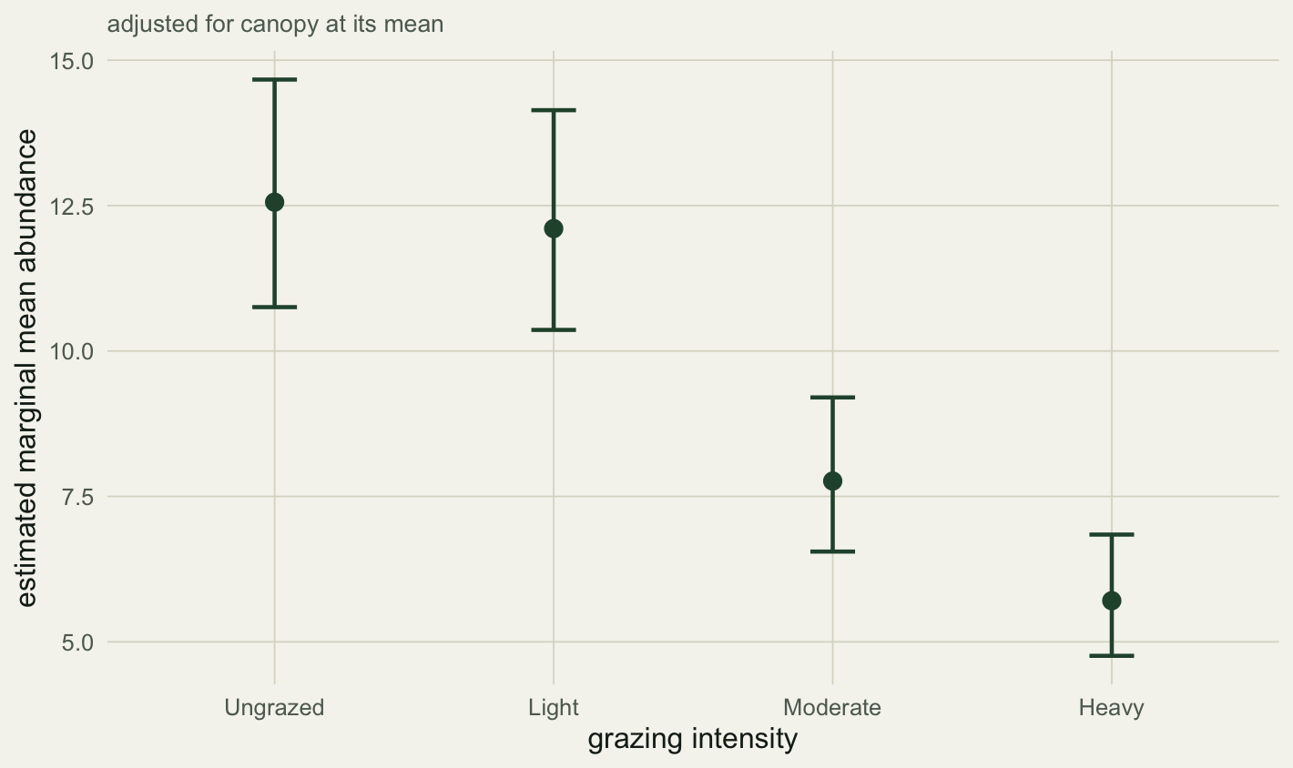
These are predicted abundances of about 12.6, 12.1, 7.8, and 5.7 from Ungrazed to Heavy, each adjusted to the mean canopy and each carrying its own interval. The intervals are built on the link scale and back-transformed, the [response-scale rule](../predicting-glm-response-scale/) from the prediction post. The whole construction is what `predict()` does internally, which is a useful check:
```{r}
#| label: emm-check
max(abs(emm$mean - predict(m, newdata = grid, type = "response")))
```
```{r}
#| label: fig-emm
#| fig-cap: "Estimated marginal mean abundance for each grazing level, adjusted for canopy at its mean, with 95% intervals."
#| fig-alt: "Four points with error bars showing predicted abundance declining from ungrazed and light, which overlap, down to moderate and heavy."
#| fig-width: 7.4
#| fig-height: 4.4
emm$graze <- factor(emm$graze, levels = lev)
ggplot(emm, aes(graze, mean)) +
  geom_errorbar(aes(ymin = lo, ymax = hi), width = .16, colour = forest, linewidth = .8) +
  geom_point(colour = forest, size = 3) +
  labs(x = "grazing intensity", y = "estimated marginal mean abundance",
       subtitle = "adjusted for canopy at its mean") +
  theme_te()
```
## Contrasts are differences of those means
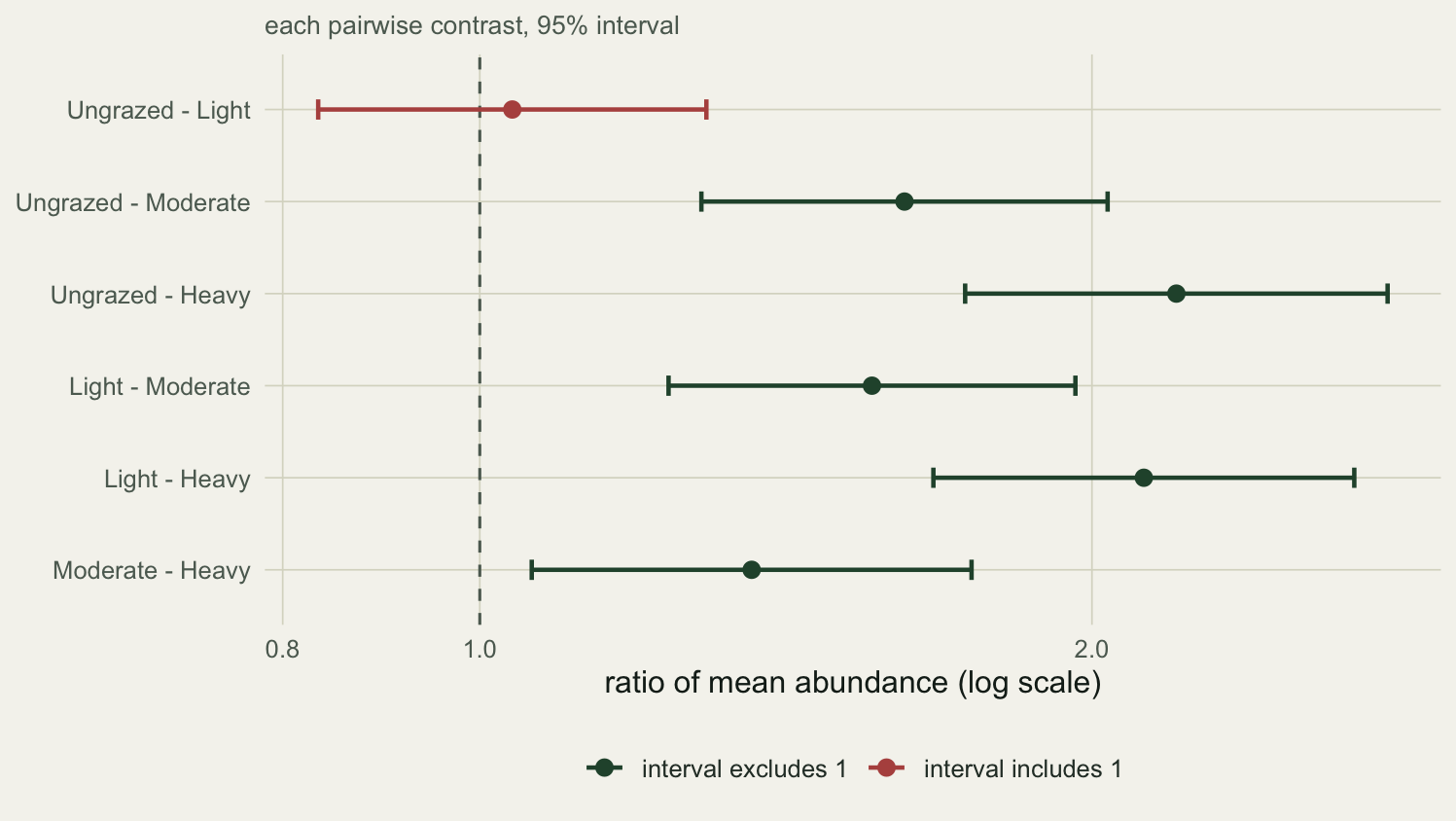
A pairwise comparison is the difference between two reference-grid rows. Subtract the two model-matrix rows to get a contrast vector, and the same two formulas give the estimate and its standard error. On a log link the difference of two log means is a log ratio, so exponentiating returns the ratio of mean abundance between the groups.
```{r}
#| label: contrasts
cb    <- combn(seq_along(lev), 2)
con   <- apply(cb, 2, function(ix){
  d <- L[ix[1], ] - L[ix[2], ]                       # contrast vector
  c(est = sum(d * b),                                # difference of log means
    se  = sqrt(as.numeric(t(d) %*% V %*% d)))        # delta-method SE
})
est   <- con["est", ]; se_c <- con["se", ]
clab  <- apply(cb, 2, function(ix) paste(lev[ix[1]], lev[ix[2]], sep = " - "))
res   <- data.frame(contrast = clab,
                    ratio = round(exp(est), 4),
                    lo    = round(exp(est - crit * se_c), 4),
                    hi    = round(exp(est + crit * se_c), 4),
                    p     = round(2 * pnorm(-abs(est / se_c)), 4))
res
```
Ungrazed and Light are within sampling noise of each other, a ratio near 1.04 whose interval spans 1. Every comparison that steps two or more levels apart shows a clear ratio: abundance under heavy grazing is about 2.2 times lower than ungrazed. The adjacent pair Moderate against Heavy sits at a ratio of 1.36 with an interval that just clears 1, which is exactly the comparison the next step will reconsider.
```{r}
#| label: fig-contrasts
#| fig-cap: "Each pairwise contrast as a ratio of mean abundance with its 95% interval, on a log scale. Intervals clear of the dashed line at one are the separable pairs."
#| fig-alt: "A forest plot of six abundance ratios with intervals. The ungrazed versus light interval crosses the reference line at one; the other five sit to its right."
#| fig-width: 7.8
#| fig-height: 4.4
R <- res
R$contrast <- factor(clab, levels = rev(clab))
R$flag <- ifelse(R$lo > 1 | R$hi < 1, "interval excludes 1", "interval includes 1")
ggplot(R, aes(ratio, contrast, colour = flag)) +
  geom_vline(xintercept = 1, colour = faint, linetype = "dashed") +
  geom_errorbarh(aes(xmin = lo, xmax = hi), height = .22, linewidth = .8) +
  geom_point(size = 2.6) +
  scale_x_log10() +
  scale_colour_manual(values = c("interval excludes 1"=forest, "interval includes 1"=aban)) +
  labs(x = "ratio of mean abundance (log scale)", y = NULL, colour = NULL,
       subtitle = "each pairwise contrast, 95% interval") +
  theme_te()
```
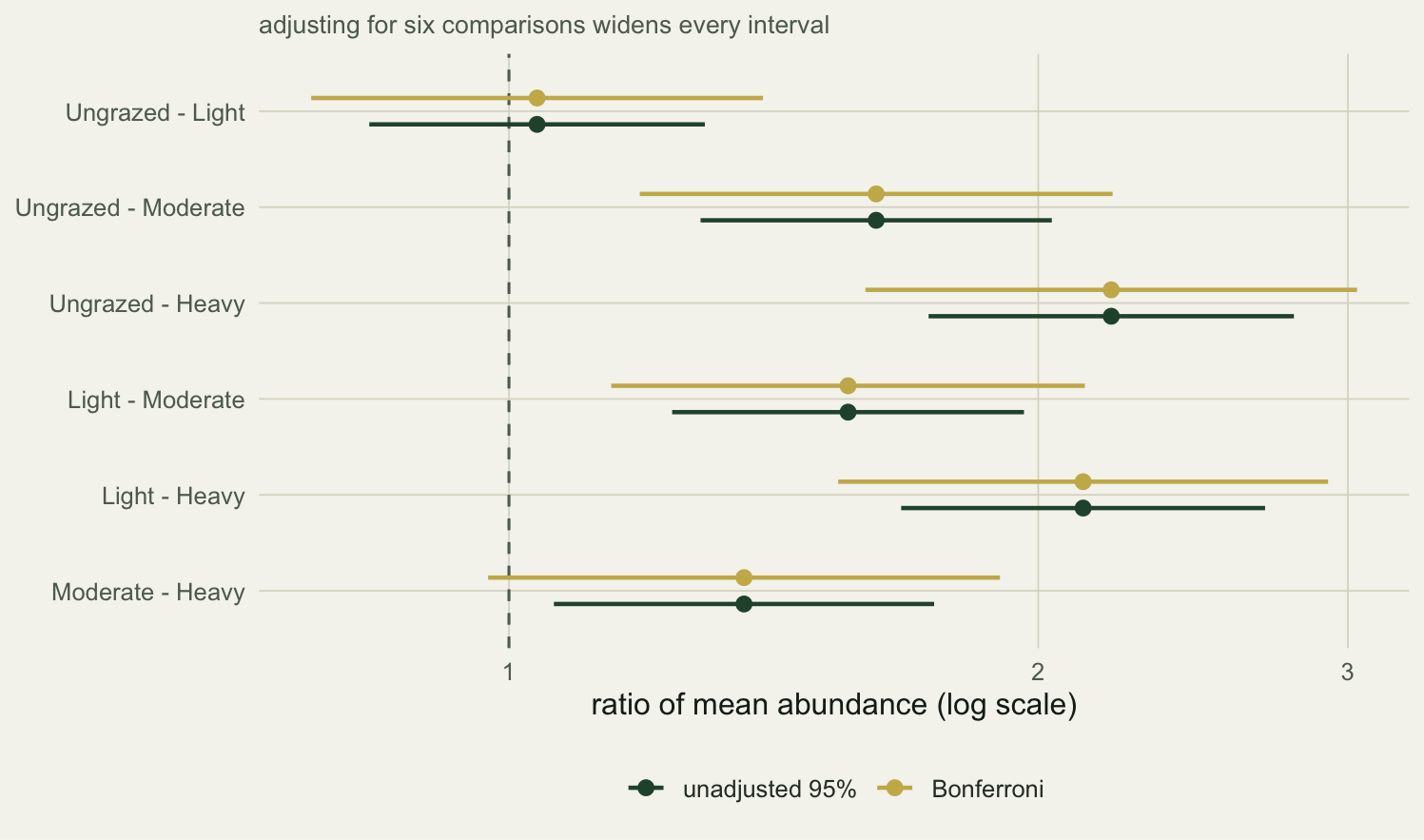
## Multiple comparisons change the verdict
Six comparisons among four groups means six chances to cross a 0.05 threshold by accident, so the raw p-values need adjustment (Hothorn, Bretz and Westfall 2008). The same `p.adjust()` the [pairwise PERMANOVA post](../pairwise-permanova/) used applies here:
```{r}
#| label: adjust
data.frame(contrast = res$contrast,
           raw  = round(res$p, 4),
           bonf = round(p.adjust(res$p, "bonferroni"), 4),
           holm = round(p.adjust(res$p, "holm"), 4))
```
The decisive pairs do not move: heavy and light grazing stay clearly separable from the ungrazed and lightly grazed plots. The borderline Moderate against Heavy is where the choice bites. Its raw p-value of 0.015 is significant, Bonferroni pushes it to 0.092 and drops it, while Holm leaves it at 0.031 and keeps it. As with the false discovery rate in the PERMANOVA post (Benjamini and Hochberg 1995), the correction is a deliberate choice with consequences, not a formality. On the interval scale the same flip looks like a widening: the multiplicity-adjusted interval for that pair now reaches back across 1.
```{r}
#| label: fig-multiplicity
#| fig-cap: "The pairwise ratios with unadjusted and Bonferroni intervals. Adjusting for six comparisons widens every interval, and the moderate-heavy interval crosses one."
#| fig-alt: "The same six ratios, each with two intervals. The Bonferroni intervals are wider than the unadjusted ones, and for moderate versus heavy the wider interval now includes one."
#| fig-width: 7.8
#| fig-height: 4.6
zb <- qnorm(1 - 0.05 / (2 * length(est)))            # Bonferroni critical value
W  <- rbind(
  data.frame(contrast = clab, ratio = exp(est),
             lo = exp(est - crit * se_c), hi = exp(est + crit * se_c), band = "unadjusted 95%"),
  data.frame(contrast = clab, ratio = exp(est),
             lo = exp(est - zb * se_c),   hi = exp(est + zb * se_c),   band = "Bonferroni"))
W$contrast <- factor(W$contrast, levels = rev(clab))
W$band     <- factor(W$band, levels = c("unadjusted 95%", "Bonferroni"))
ggplot(W, aes(ratio, contrast, colour = band)) +
  geom_vline(xintercept = 1, colour = faint, linetype = "dashed") +
  geom_errorbarh(aes(xmin = lo, xmax = hi), height = 0, linewidth = .8,
                 position = position_dodge(width = .55)) +
  geom_point(size = 2.4, position = position_dodge(width = .55)) +
  scale_x_log10() +
  scale_colour_manual(values = c("unadjusted 95%"=forest, "Bonferroni"=gold)) +
  labs(x = "ratio of mean abundance (log scale)", y = NULL, colour = NULL,
       subtitle = "adjusting for six comparisons widens every interval") +
  theme_te()
```
## Check it, then let a package carry it
Hand-built contrasts are worth validating against something independent. Releveling so Moderate is the reference makes the `grazeHeavy` coefficient the Moderate-to-Heavy difference directly, which should match the contrast above up to sign:
```{r}
#| label: validate
mm <- glm.nb(abund ~ graze + canopy, data = transform(D, graze = relevel(graze, ref = "Moderate")))
c(by_hand_log_ratio = unname(sum((L[3,] - L[4,]) * b)),
  relevel_coef      = unname(coef(mm)["grazeHeavy"]))
```
They agree to sign, since one is Moderate minus Heavy and the other Heavy minus Moderate. Once the mechanics are clear, `emmeans` (Lenth 2016) and `marginaleffects` do all of this from one call: a reference grid, contrasts as linear combinations, delta-method intervals, and the Tukey adjustment that is the standard choice for all-pairwise comparisons rather than the Bonferroni used here for transparency. They also back-transform to the response scale and carry interactions, so the grouped slopes from the [interaction post](../interaction-terms-glm/) can be compared the same way. The by-hand version is for seeing what those functions return.
## References
Benjamini Y, Hochberg Y (1995). Controlling the False Discovery Rate: A Practical and Powerful Approach to Multiple Testing. *Journal of the Royal Statistical Society B* 57(1):289-300. doi:10.1111/j.2517-6161.1995.tb02031.x
Hothorn T, Bretz F, Westfall P (2008). Simultaneous Inference in General Parametric Models. *Biometrical Journal* 50(3):346-363. doi:10.1002/bimj.200810425
Lenth RV (2016). Least-Squares Means: The R Package lsmeans. *Journal of Statistical Software* 69(1):1-33. doi:10.18637/jss.v069.i01
Searle SR, Speed FM, Milliken GA (1980). Population Marginal Means in the Linear Model: An Alternative to Least Squares Means. *The American Statistician* 34(4):216-221. doi:10.1080/00031305.1980.10483031