library(ggplot2)

te_paper  <- "#f5f4ee"
te_ink    <- "#16241d"
te_body   <- "#2c3a31"
te_forest <- "#275139"
te_rust   <- "#b5534e"
te_gold   <- "#c9b458"
te_line   <- "#dad9ca"
te_sage   <- "#93a87f"

theme_datasheet <- function() {
  theme_minimal(base_size = 12) +
    theme(plot.background  = element_rect(fill = te_paper, colour = NA),
          panel.background = element_rect(fill = te_paper, colour = NA),
          panel.grid.major = element_line(colour = te_line, linewidth = 0.3),
          panel.grid.minor = element_blank(),
          text             = element_text(colour = te_body),
          plot.title       = element_text(colour = te_ink, face = "bold"),
          plot.subtitle    = element_text(colour = te_body),
          axis.text        = element_text(colour = te_body),
          strip.text       = element_text(colour = te_ink, face = "bold"))
}Checking a phylogenetic regression’s branch lengths
R
phylogenetics
comparative methods
model diagnostics
simulation
ecology tutorial
Wrong branch lengths make PGLS find slopes that are not there. How often the Garland check notices, on coalescent and Yule trees of 20 to 80 species, in R.
Forty species of warbler, a published time-calibrated tree trimmed to them, and a regression of clutch size on body mass fitted as phylogenetic generalised least squares. The slope comes back with a small p value. The tree was dated for another purpose, its branch lengths are in millions of years, and the analysis assumes that both traits changed in proportion to that time. If they changed mostly at speciation instead, the covariance the regression used is the wrong one, and the p value was computed against a null that does not describe the data.
This site has the pieces of that problem but not the problem. Independent contrasts: Felsenstein’s method introduces the standard diagnostic in its section on checking the branch lengths, the absolute standardised contrasts plotted against their standard deviations, and draws it once, on a tree that is right; its caption reads that a flat cloud means the standardisation is working. Phylogenetic generalised least squares measures what ignoring the tree does to the Type I error, again with the correct tree in the model. Brownian motion or Ornstein-Uhlenbeck? lists among its honest limits that an error in the branch lengths near the tips was not simulated. Checking a community phylogenetics analysis does set every branch to one, but for a community clustering index, not a regression.
This post breaks the branch lengths under a regression and measures three things: how often PGLS then rejects a slope that is truly zero, how often the Garland check notices, and whether it notices in the datasets that were actually damaged. The first result is not new. Diaz-Uriarte and Garland (1996, 1998) measured the Type I error of independent contrasts under departures from Brownian motion and under branch length errors, and found that distorted lengths often inflated it. They also found that checking the lengths with the Garland, Harvey and Ives (1992) diagnostic and transforming them when it failed brought the error rates back under control; the switch repair below is a cut-down version of that procedure, restricted to three fixed sets of lengths. What follows is a demonstration of both on hand-built trees. The pieces added here are the detection rate of the check conditional on a false positive, how it changes between 20 and 80 species, and how both depend on the tree generator. As in the Ornstein-Uhlenbeck post, no comparative methods package is used: trees, covariance matrices, contrasts and fits are all base R.
One topology, three sets of branch lengths
Every dataset starts from a random topology built backwards from the tips by merging a uniformly chosen pair of lineages, the construction used in the Ornstein-Uhlenbeck post. Two rules for the waiting times give the dates. While k lineages remain, the next merge comes after an exponential time with rate k(k - 1)/2 on a coalescent-like tree, which crowds most splits close to the tips, or with rate k on a Yule-like tree. Node ages are rescaled so the root sits at one.
The same topology then carries three sets of branch lengths. Dated lengths are differences of node ages. Equal lengths set every branch to one, which is the covariance of a trait that changes only at speciation events. Grafen’s lengths give each node a height equal to the number of tips below it minus one, scaled so the root is at one: that is the recipe of Grafen (1989) with his power rho fixed at one, and it is a common fallback for a tree that has a topology and no dates.
The covariance matrix is the shared path from the root, built from a node-by-tip membership matrix weighted by the square root of each branch length. Contrasts come from Felsenstein’s recursion, taking the merges in the order they were made so that both children are finished before their parent: each internal node is given the weighted mean of its two children, and its own branch is lengthened by the product of the children’s lengths over their sum. PGLS is least squares after whitening with the Cholesky factor of the covariance. The Garland check is the one drawn in the contrasts post, the Pearson correlation between the absolute standardised contrasts and their standard deviations, tested at five per cent, as Garland, Harvey and Ives (1992) proposed it.
sim_topology <- function(n_tip, shape = c("coalescent", "yule")) {
  shape <- match.arg(shape)
  active <- seq_len(n_tip); next_id <- n_tip + 1L; age <- 0
  node_age <- numeric(2 * n_tip - 1)
  merges <- matrix(0L, n_tip - 1, 3)
  for (i in seq_len(n_tip - 1)) {
    k <- length(active)
    age <- age + rexp(1, rate = if (shape == "yule") k else k * (k - 1) / 2)
    pick <- active[sample.int(k, 2)]
    node_age[next_id] <- age
    merges[i, ] <- c(pick, next_id)
    active <- c(active[!active %in% pick], next_id)
    next_id <- next_id + 1L
  }
  parent <- integer(2 * n_tip - 1)
  parent[merges[, 1]] <- merges[, 3]; parent[merges[, 2]] <- merges[, 3]
  clade_size <- c(rep(1L, n_tip), integer(n_tip - 1))
  for (i in seq_len(n_tip - 1))
    clade_size[merges[i, 3]] <- clade_size[merges[i, 1]] + clade_size[merges[i, 2]]
  list(n = n_tip, merges = merges, parent = parent,
       age = node_age / age, clade_size = clade_size)
}

# branch lengths: dated tree, all branches one, or Grafen's heights (rho = 1)
edge_lengths <- function(tree, scheme = c("time", "equal", "grafen")) {
  scheme <- match.arg(scheme)
  below_root <- which(tree$parent > 0)
  len <- numeric(2 * tree$n - 1)
  if (scheme == "equal") {
    len[below_root] <- 1
  } else {
    height <- if (scheme == "time") tree$age else (tree$clade_size - 1) / (tree$n - 1)
    len[below_root] <- height[tree$parent[below_root]] - height[below_root]
  }
  len
}

# shared path from the root: rows of 'member' mark the tips below each node
tree_vcv <- function(tree, len) {
  member <- matrix(0, 2 * tree$n - 1, tree$n)
  member[cbind(seq_len(tree$n), seq_len(tree$n))] <- 1
  for (i in seq_len(tree$n - 1)) {
    m <- tree$merges[i, ]
    member[m[3], ] <- member[m[1], ] + member[m[2], ]
  }
  crossprod(member * sqrt(len))
}

pagel_vcv <- function(vcv_mat, lambda) {
  out <- lambda * vcv_mat; diag(out) <- diag(vcv_mat); out
}

# Pagel's kappa: every branch length raised to the power kappa. Built once per
# tree: 'clade' marks the nodes below each node, 'mrca' the common ancestor of
# each pair of tips, so a new kappa only needs the node depths.
kappa_setup <- function(tree) {
  clade <- diag(2 * tree$n - 1)
  mrca <- diag(seq_len(tree$n))
  tips <- seq_len(tree$n)
  for (i in seq_len(tree$n - 1)) {
    m <- tree$merges[i, ]
    clade[m[3], ] <- clade[m[3], ] + clade[m[1], ] + clade[m[2], ]
    in_a <- clade[m[1], tips] > 0; in_b <- clade[m[2], tips] > 0
    mrca[in_a, in_b] <- m[3]; mrca[in_b, in_a] <- m[3]
  }
  list(n = tree$n, clade = clade, mrca = mrca)
}

kappa_vcv <- function(ks, len, power_k) {
  pos <- len > 0
  len_k <- numeric(length(len)); len_k[pos] <- exp(power_k * log(len[pos]))
  depth <- drop(crossprod(ks$clade, len_k))
  matrix(depth[ks$mrca], ks$n, ks$n)
}

# Felsenstein's contrasts by recursion, one column per trait
pic_contrasts <- function(tree, len, traits) {
  traits <- as.matrix(traits)
  v <- len
  val <- rbind(traits, matrix(NA, tree$n - 1, ncol(traits)))
  contrast <- matrix(0, tree$n - 1, ncol(traits)); sd_con <- numeric(tree$n - 1)
  for (i in seq_len(tree$n - 1)) {
    a <- tree$merges[i, 1]; b <- tree$merges[i, 2]; p <- tree$merges[i, 3]
    s <- v[a] + v[b]
    contrast[i, ] <- (val[a, ] - val[b, ]) / sqrt(s); sd_con[i] <- sqrt(s)
    val[p, ] <- (val[a, ] * v[b] + val[b, ] * v[a]) / s
    v[p] <- v[p] + v[a] * v[b] / s
  }
  list(contrast = contrast, sd = sd_con)
}

# PGLS by Cholesky whitening; profile log-likelihood with sigma squared out
pgls_fit <- function(vcv_mat, x, y) {
  up <- chol(vcv_mat)
  xw <- backsolve(up, cbind(1, x), transpose = TRUE)
  yw <- backsolve(up, y, transpose = TRUE)
  fit <- lm.fit(xw, yw); n_sp <- length(y); rss <- sum(fit$residuals^2)
  se_b <- sqrt(rss / (n_sp - 2) * chol2inv(chol(crossprod(xw)))[2, 2])
  b_hat <- unname(fit$coefficients[2])
  c(slope = b_hat, p = 2 * pt(-abs(b_hat / se_b), n_sp - 2),
    loglik = -n_sp / 2 * log(rss / n_sp) - sum(log(diag(up))))
}

# the Garland check: |standardised contrast| against its standard deviation
garland_check <- function(contrast, sd_con) {
  ct <- cor.test(abs(contrast), sd_con)
  c(r = unname(ct$estimate), p = ct$p.value)
}
Three checks come before any measurement. For any data and any set of branch lengths, the regression of contrasts through the origin and PGLS give the same slope, so a disagreement would expose an error in one of the two routes. And when a trait is simulated on the same lengths that standardise its contrasts, those contrasts are independent standard normal variates, so their mean square should be one. Finally, Pagel’s (1999) kappa, which raises every branch length to a power and is used as a repair further down, must return the equal lengths at a power of zero and the dated lengths at a power of one.
set.seed(3101)
chk_tree <- sim_topology(30, "coalescent")
chk_x <- rnorm(30); chk_y <- rnorm(30)
slope_gap <- max(vapply(c("time", "equal", "grafen"), function(sch) {
  len <- edge_lengths(chk_tree, sch)
  pc <- pic_contrasts(chk_tree, len, cbind(chk_x, chk_y))
  b_pic <- sum(pc$contrast[, 1] * pc$contrast[, 2]) / sum(pc$contrast[, 1]^2)
  abs(b_pic - pgls_fit(tree_vcv(chk_tree, len), chk_x, chk_y)["slope"])
}, 0))

n_var_chk <- 400
set.seed(3102)
con_sq <- t(vapply(seq_len(n_var_chk), function(i) {
  tr <- sim_topology(40, "coalescent")
  vapply(c("time", "equal"), function(sch) {
    len <- edge_lengths(tr, sch)
    trait <- drop(t(chol(tree_vcv(tr, len))) %*% rnorm(40))
    mean(pic_contrasts(tr, len, trait)$contrast^2)
  }, 0)
}, numeric(2)))
msq_time <- mean(con_sq[, 1]); msq_equal <- mean(con_sq[, 2])
msq_se <- apply(con_sq, 2, sd) / sqrt(n_var_chk)
msq_z <- max(abs(colMeans(con_sq) - 1) / msq_se)

chk_ks <- kappa_setup(chk_tree); chk_time <- edge_lengths(chk_tree, "time")
kappa_gap <- max(abs(kappa_vcv(chk_ks, chk_time, 0) - tree_vcv(chk_tree, edge_lengths(chk_tree, "equal"))),
                 abs(kappa_vcv(chk_ks, chk_time, 1) - tree_vcv(chk_tree, chk_time)))
On a 30 species tree the largest slope difference between contrasts and PGLS across the three sets of lengths is 9.4e-14, which is rounding error. Over 400 trees of 40 species the mean squared contrast is 1.002 for traits simulated and standardised on dated lengths and 1.015 on equal lengths, with Monte Carlo standard errors of 0.011 and 0.012; the larger departure from one is 1.3 standard errors. The kappa covariance differs from the equal-length and dated covariances at the two ends by at most 2.2e-16. The recursion, the covariance matrix and the fit agree with each other and with the theory.
One dataset with the wrong lengths
The warbler analysis in miniature: a coalescent-like tree of 40 species, both traits evolved independently by Brownian motion on equal branch lengths, and PGLS fitted with the dated lengths. The chunk draws datasets until the first one in which the dated analysis rejects a zero slope, which is how this example was chosen.
n_demo <- 40
set.seed(8801)
n_tried <- 0
repeat {
  n_tried <- n_tried + 1
  demo_tree <- sim_topology(n_demo, "coalescent")
  len_true <- edge_lengths(demo_tree, "equal"); len_used <- edge_lengths(demo_tree, "time")
  chol_true <- t(chol(tree_vcv(demo_tree, len_true)))
  demo_x <- drop(chol_true %*% rnorm(n_demo)); demo_y <- drop(chol_true %*% rnorm(n_demo))
  fit_used <- pgls_fit(tree_vcv(demo_tree, len_used), demo_x, demo_y)
  if (fit_used["p"] < 0.05) break
}
fit_true <- pgls_fit(tree_vcv(demo_tree, len_true), demo_x, demo_y)
pic_used <- pic_contrasts(demo_tree, len_used, demo_x)
pic_true <- pic_contrasts(demo_tree, len_true, demo_x)
g_used <- garland_check(pic_used$contrast, pic_used$sd)
g_true <- garland_check(pic_true$contrast, pic_true$sd)
sd_ratio_used <- max(pic_used$sd) / min(pic_used$sd)
The first false positive came at draw 3. With the dated lengths PGLS returns a slope of 1.149 and a p value of 0.00013. With the lengths the traits evolved on, the same data give 0.075 and 0.738. The traits are unrelated, so the first result is a false positive.
The check on the predictor, computed with the dated lengths the analyst has, gives a correlation of -0.547 with a p value of 0.0003: it fires. With the true lengths it gives -0.228 and 0.162. The left panel shows why. On the dated coalescent-like tree the largest contrast standard deviation is 48 times the smallest, because sister species that split very recently are joined by very short branches. Under equal lengths those sisters differ by as much as any other pair, so dividing their difference by a tiny standard deviation produces the huge standardised contrasts at the left of the panel.
panel_lev <- c("dated lengths (used)", "equal lengths (true)")
worked_df <- rbind(
  data.frame(panel = panel_lev[1], sd_con = pic_used$sd, abs_con = abs(pic_used$contrast[, 1])),
  data.frame(panel = panel_lev[2], sd_con = pic_true$sd, abs_con = abs(pic_true$contrast[, 1])))
worked_df$panel <- factor(worked_df$panel, levels = panel_lev)
ggplot(worked_df, aes(sd_con, abs_con)) +
  geom_point(aes(colour = panel), size = 2, alpha = 0.8, show.legend = FALSE) +
  geom_smooth(method = "lm", formula = y ~ x, se = FALSE, colour = te_ink, linewidth = 0.7) +
  scale_colour_manual(values = c(te_rust, te_forest)) +
  facet_wrap(~panel, scales = "free") +
  labs(x = "standard deviation of the contrast", y = "absolute standardised contrast",
       title = "The check on the predictor, same clade, two sets of lengths",
       subtitle = "line: least squares fit through the cloud") +
  theme_datasheet()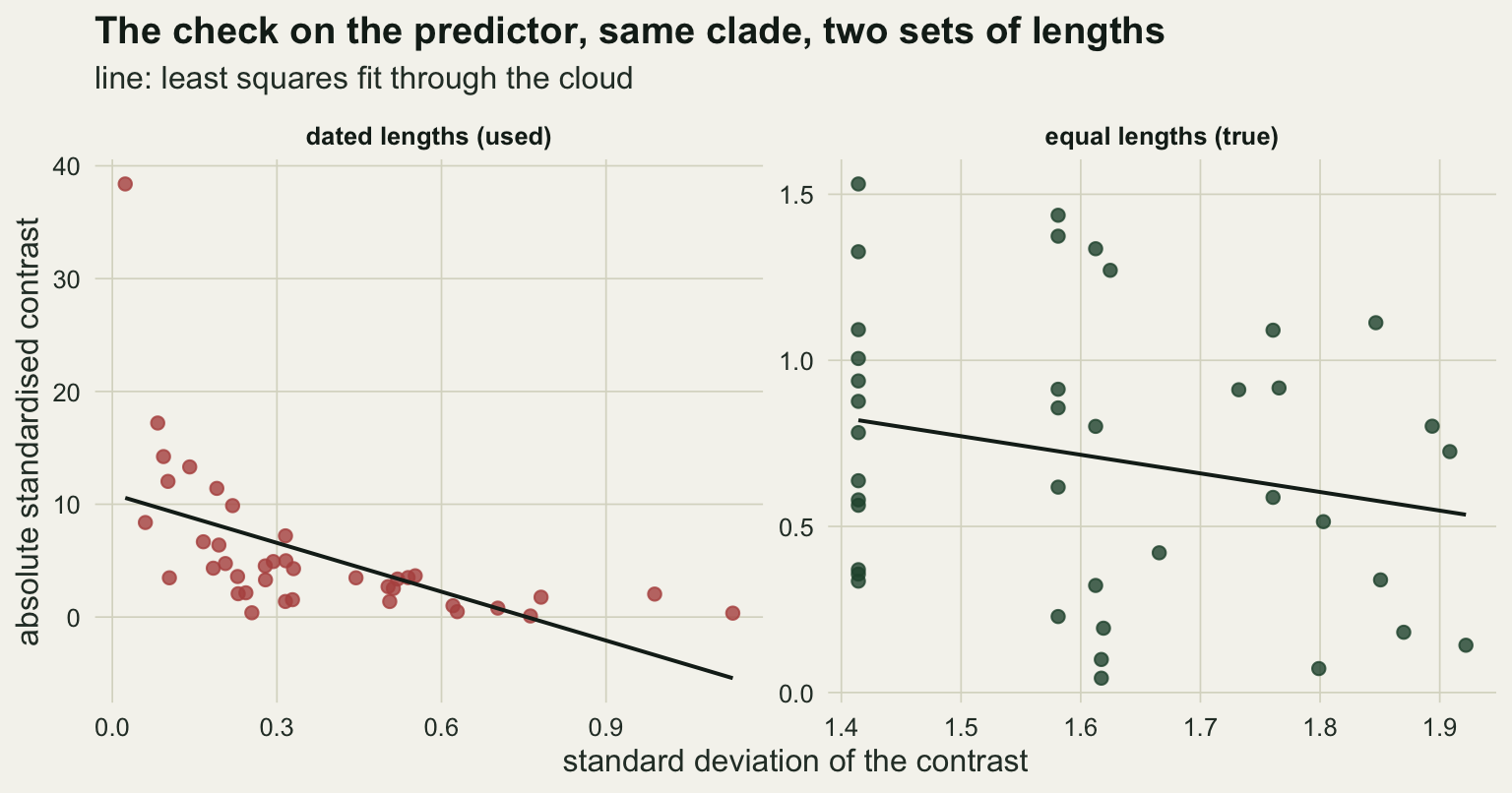
How often the wrong lengths find a slope
The grid was fixed before any rate was looked at. The truth is one of three covariance models: dated lengths, equal lengths, or Pagel’s (1999) lambda of 0.5 on the dated tree, which halves every shared path while keeping the tip variances. There are two generators, 20, 40 and 80 species, and 500 null datasets per cell with a fresh tree for each. Both traits always evolve independently, so the true slope is zero. Every dataset is analysed with all three sets of lengths and with lambda and kappa estimated, so comparisons between analyses are paired.
n_grid     <- c(20, 40, 80)
shapes     <- c("coalescent", "yule")
truths     <- c("time", "equal", "lambda")
lambda_true <- 0.5
n_rep      <- 500     # fixed before any rate was inspected
alpha_lev  <- 0.05
schemes    <- c("time", "equal", "grafen")

one_dataset <- function(n_sp, shape, truth) {
  tr <- sim_topology(n_sp, shape)
  lens <- lapply(setNames(schemes, schemes), function(sch) edge_lengths(tr, sch))
  vcvs <- lapply(lens, function(len) tree_vcv(tr, len))
  vcv_truth <- switch(truth, time = vcvs$time, equal = vcvs$equal,
                      lambda = pagel_vcv(vcvs$time, lambda_true))
  chol_truth <- t(chol(vcv_truth))
  x <- drop(chol_truth %*% rnorm(n_sp)); y <- drop(chol_truth %*% rnorm(n_sp))
  out <- numeric(0)
  for (sch in schemes) {
    fit <- pgls_fit(vcvs[[sch]], x, y)
    pc <- pic_contrasts(tr, lens[[sch]], cbind(x, y))
    b0 <- sum(pc$contrast[, 1] * pc$contrast[, 2]) / sum(pc$contrast[, 1]^2)
    res_con <- pc$contrast[, 2] - b0 * pc$contrast[, 1]
    gx <- garland_check(pc$contrast[, 1], pc$sd)
    gy <- garland_check(pc$contrast[, 2], pc$sd)
    gr <- garland_check(res_con, pc$sd)
    out <- c(out, setNames(c(fit["p"], fit["loglik"], gx, gy["r"], gy["p"], gr["p"]),
                           paste(sch, c("p", "ll", "rx", "px", "ry", "py", "pr"), sep = "_")))
  }
  prof <- function(lam) pgls_fit(pagel_vcv(vcvs$time, lam), x, y)["loglik"]
  opt <- optimize(prof, c(0, 1), maximum = TRUE)
  cand <- c(0, opt$maximum, 1)
  lam_hat <- cand[which.max(vapply(cand, prof, 0))]
  ks <- kappa_setup(tr)
  prof_k <- function(kap) pgls_fit(kappa_vcv(ks, lens$time, kap), x, y)["loglik"]
  opt_k <- optimize(prof_k, c(0, 1), maximum = TRUE, tol = 0.005)
  cand_k <- c(0, opt_k$maximum, 1)
  kap_hat <- cand_k[which.max(vapply(cand_k, prof_k, 0))]
  c(out, lambda_hat = lam_hat,
    lambda_p = unname(pgls_fit(pagel_vcv(vcvs$time, lam_hat), x, y)["p"]),
    kappa_hat = kap_hat,
    kappa_p = unname(pgls_fit(kappa_vcv(ks, lens$time, kap_hat), x, y)["p"]))
}

cells <- expand.grid(truth = truths, shape = shapes, n = n_grid, stringsAsFactors = FALSE)
set.seed(20260908)
sims <- do.call(rbind, lapply(seq_len(nrow(cells)), function(i) {
  runs <- t(replicate(n_rep, one_dataset(cells$n[i], cells$shape[i], cells$truth[i])))
  data.frame(cells[rep(i, n_rep), ], runs, row.names = NULL)
}))

rates <- do.call(rbind, lapply(split(sims, list(sims$shape, sims$truth, sims$n)), function(d) {
  do.call(rbind, lapply(schemes, function(sch) {
    rej <- d[[paste0(sch, "_p")]] < alpha_lev
    fx  <- d[[paste0(sch, "_px")]] < alpha_lev
    fxy <- fx | d[[paste0(sch, "_py")]] < alpha_lev
    data.frame(shape = d$shape[1], truth = d$truth[1], n = d$n[1], analyst = sch,
               fpr = mean(rej), n_fp = sum(rej), fires = mean(fx),
               fires_fp = mean(fx[rej]), fires_ok = mean(fx[!rej]),
               fires_xy = mean(fxy), fires_xy_fp = mean(fxy[rej]),
               fires_res = mean(d[[paste0(sch, "_pr")]] < alpha_lev))
  }))
}))
rates$mcse <- sqrt(rates$fpr * (1 - rates$fpr) / n_rep)
rt <- function(shape, truth, analyst, n, what = "fpr")
  rates[rates$shape == shape & rates$truth == truth & rates$analyst == analyst & rates$n == n, what]
correct <- rates[rates$truth == rates$analyst, ]
mcse_nom <- sqrt(alpha_lev * (1 - alpha_lev) / n_rep)
When the analyst’s lengths match the truth, the rejection rate lies between 2.8 and 6.2 per cent across the 12 matched cells, with a Monte Carlo standard error of 1.0 percentage points near five per cent.
The two errors named at the start are large on coalescent-like trees. Dated lengths on equal-length truth reject a true zero slope in 31.2, 41.2 and 47.2 per cent of datasets at 20, 40 and 80 species; equal lengths on dated truth in 24.4, 32.8 and 42.0 per cent. The standard errors of these rates are at most 2.2 points. On Yule-like trees the first error is of similar size (28.2 to 41.0 per cent), but the reverse is much milder, 9.2, 11.6 and 10.6 per cent: a Yule-like tree has no crowd of very short tip branches, so ignoring its dates distorts the covariance less. Dated lengths on lambda truth reach 54.2 per cent at 80 species on coalescent-like trees.
In those four large errors the rate rises with the number of species. More species do not dilute a wrong covariance matrix; they make the test more confident in it. Equal lengths on lambda truth stay between 6.2 and 8.4 per cent, and Grafen’s lengths, never the truth here, land between 5.0 and 18.0 per cent, which makes them the case worth a closer look below.
truth_lab <- c(time = "truth: dated lengths", equal = "truth: equal lengths",
               lambda = "truth: lambda 0.5 on dated")
analyst_lab <- c(time = "dated", equal = "equal", grafen = "Grafen")
fpr_df <- rates
fpr_df$truth_f <- factor(truth_lab[fpr_df$truth], levels = truth_lab)
fpr_df$analyst_f <- factor(analyst_lab[fpr_df$analyst], levels = analyst_lab)
shape_lab <- c(coalescent = "coalescent-like tree", yule = "Yule-like tree")
fpr_df$shape_f <- factor(shape_lab[fpr_df$shape], levels = shape_lab)
ggplot(fpr_df, aes(n, fpr, colour = analyst_f)) +
  geom_hline(yintercept = alpha_lev, linetype = "dashed", colour = te_body, linewidth = 0.5) +
  geom_errorbar(aes(ymin = fpr - 2 * mcse, ymax = fpr + 2 * mcse), width = 4, linewidth = 0.4) +
  geom_line(linewidth = 0.9) + geom_point(size = 2) +
  scale_colour_manual(values = c(te_forest, te_rust, te_gold), name = "lengths the analyst used") +
  scale_x_continuous(breaks = n_grid) +
  facet_grid(shape_f ~ truth_f) +
  labs(x = "species", y = "rejection rate, true slope zero",
       title = "Wrong lengths reject a true null",
       subtitle = "dashed line: five per cent; bars: two Monte Carlo standard errors") +
  theme_datasheet() + theme(legend.position = "bottom")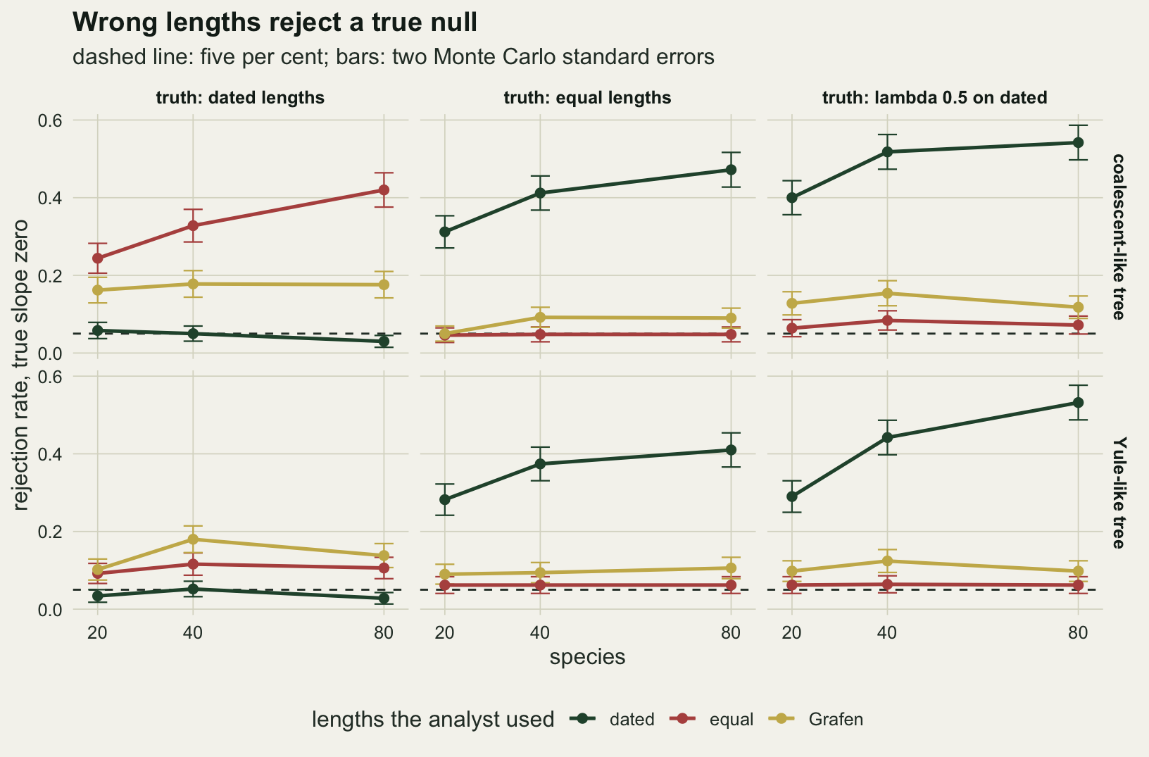
The check mostly notices the tree, not the damaged dataset
The check is run on the predictor contrasts computed with the lengths the analyst used, the only tree the analyst has. Three errors are followed: the two from the previous section and Grafen’s lengths on dated truth. The number that matters is not how often the check fires overall but how often it fires in the datasets where PGLS gave a false positive, set against the datasets where it did not.
errors <- data.frame(
  label = c("dated used, equal true", "equal used, dated true", "Grafen used, dated true"),
  truth = c("equal", "time", "time"), analyst = c("time", "equal", "grafen"))
detect_df <- do.call(rbind, lapply(seq_len(nrow(errors)), function(k) {
  err_rows <- rates[rates$truth == errors$truth[k] & rates$analyst == errors$analyst[k], ]
  rbind(data.frame(error = errors$label[k], shape = err_rows$shape, n = err_rows$n,
                   which = "all datasets", rate = err_rows$fires),
        data.frame(error = errors$label[k], shape = err_rows$shape, n = err_rows$n,
                   which = "false positives", rate = err_rows$fires_fp),
        data.frame(error = errors$label[k], shape = err_rows$shape, n = err_rows$n,
                   which = "no false positive", rate = err_rows$fires_ok))
}))
detect_df$error <- factor(detect_df$error, levels = errors$label)
detect_df$shape_f <- factor(c(coalescent = "coalescent-like tree", yule = "Yule-like tree")[detect_df$shape],
                            levels = c("coalescent-like tree", "Yule-like tree"))
detect_df$which <- factor(detect_df$which,
                          levels = c("all datasets", "false positives", "no false positive"))
fp_min <- min(rates$n_fp[rates$shape == "coalescent" & rates$truth == "equal" & rates$analyst == "time"])
se_cond_max <- sqrt(0.25 / fp_min)
head_err <- rates[rates$shape == "coalescent" & rates$truth == "equal" & rates$analyst == "time", ]
gap_cond <- head_err$fires_fp - head_err$fires_ok
gap_se <- sqrt(head_err$fires_fp * (1 - head_err$fires_fp) / head_err$n_fp +
               head_err$fires_ok * (1 - head_err$fires_ok) / (n_rep - head_err$n_fp))
err_cells <- do.call(rbind, lapply(seq_len(nrow(errors)), function(k)
  rates[rates$truth == errors$truth[k] & rates$analyst == errors$analyst[k], ]))
err_cells$gap <- err_cells$fires_fp - err_cells$fires_ok
err_cells$gap_se <- sqrt(err_cells$fires_fp * (1 - err_cells$fires_fp) / err_cells$n_fp +
                         err_cells$fires_ok * (1 - err_cells$fires_ok) / (n_rep - err_cells$n_fp))
err_cells$z <- err_cells$gap / err_cells$gap_se
n_within <- sum(abs(err_cells$z) < 2)
gap_at <- function(shape, truth, analyst, n, what = "gap") err_cells[err_cells$shape == shape &
  err_cells$truth == truth & err_cells$analyst == analyst & err_cells$n == n, what]
n_gap_pos <- sum(err_cells$z >= 2); n_gap_neg <- sum(err_cells$z <= -2)
xy_correct <- range(correct$fires_xy); x_correct <- range(correct$fires)
For dated lengths on equal-length truth on coalescent-like trees, the check fires in 47.0, 82.8 and 95.8 per cent of all datasets at 20, 40 and 80 species. Among the false positives it fires in 44.2, 79.6 and 92.8 per cent: about eight in ten at 40 species and fewer than half at 20. For the reverse error the conditional rates are 39.3, 76.2 and 96.2 per cent. The smallest number of false positives behind any of the first three rates is 156, so their Monte Carlo standard error is at most 4.0 points.
The comparison with the undamaged datasets is the finding. In the first error the firing rate among false positives minus the rate among the other datasets is -4.0, -5.4 and -5.7 points, with standard errors of 4.8, 3.5 and 1.8 points. On coalescent-like trees this error does not make the check more likely to fire on a damaged dataset, and at 80 species it makes it less likely. Across all 18 cells of the figure (three errors, two generators, three sizes) the same gap is within two standard errors of zero in 14. It is more than two standard errors above zero in 3, all on Yule-like trees: the first error at 20 species (+28.3 points, the check firing in 77.3 per cent of false positives against 49.0 per cent of the rest) and at 40 species (+5.9), and the reverse error at 20 species (+15.7). It is more than two standard errors below zero only in the coalescent cell at 80 species above. With 18 comparisons, chance alone would put an expected 0.8 cells beyond two standard errors; the first error on Yule-like trees at 20 species, 6.4 standard errors from zero, and the coalescent cell at 80 species, at -3.1, are the two that chance does not plausibly explain. The reading that fits most of the grid is that the check detects that the lengths are wrong for the trait, a property shared by every dataset on such a tree, while whether a given dataset then produces a false positive is a separate draw that the wrong lengths have biased; on small Yule-like trees the two are linked. For the reverse error on Yule-like trees it fires in at most 39.2 per cent of datasets, which matches the milder damage there.
Running the check on both traits, and calling it fired if either correlation is significant, raises detection for the first error at 20 species on coalescent-like trees from 47.0 to 66.8 per cent. The price is false alarms: with the correct lengths the two-trait version fires in 7.0 to 10.8 per cent of datasets, against 2.8 to 5.6 per cent for the predictor alone. The check on residual contrasts, from the contrast regression through the origin, fires in 47.6 per cent at 20 species, no better than the predictor alone.
ggplot(detect_df, aes(n, rate, colour = which)) +
  geom_hline(yintercept = alpha_lev, linetype = "dashed", colour = te_body, linewidth = 0.5) +
  geom_line(linewidth = 0.9) + geom_point(size = 2) +
  scale_colour_manual(values = c(te_ink, te_rust, te_gold), name = NULL) +
  scale_x_continuous(breaks = n_grid) +
  scale_y_continuous(limits = c(0, 1)) +
  facet_grid(shape_f ~ error) +
  labs(x = "species", y = "share of datasets where the check fires",
       title = "False positives are mostly no easier to spot",
       subtitle = "dashed line: five per cent") +
  theme_datasheet() + theme(legend.position = "bottom")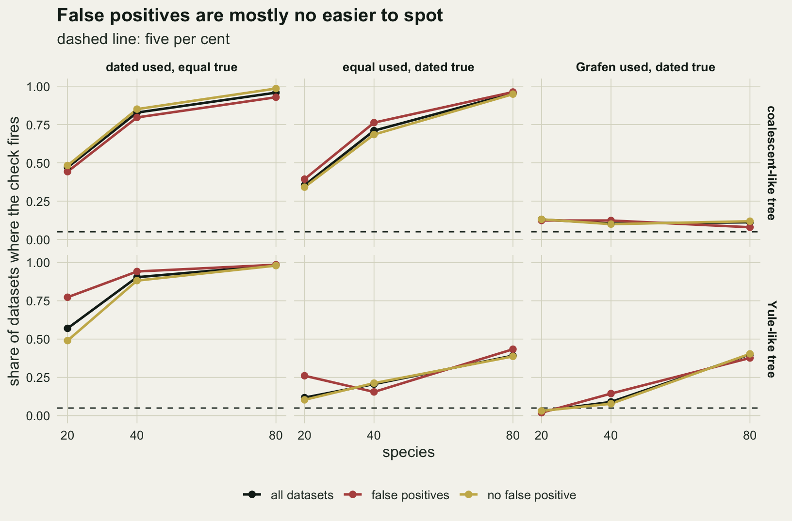
Grafen’s lengths mostly slip past the check
graf <- rates[rates$truth == "time" & rates$analyst == "grafen", ]
graf_c <- graf[graf$shape == "coalescent", ]; graf_y <- graf[graf$shape == "yule", ]
On dated truth with coalescent-like trees, Grafen’s lengths reject a true zero slope in 16.2 to 17.8 per cent of datasets, three times the nominal rate or more, and the rate does not fall with species. The check on the predictor fires in 10.4 to 13.0 per cent of those datasets, and on either trait in 21.2 to 22.2 per cent, well below the rates the other two errors reach at 40 and 80 species. At 80 species the dated-on-equal error sets off the check nearly every time; this error, with a smaller but still severe inflation, sets it off in about one dataset in ten, against 2.8 to 5.6 per cent for the predictor check with the correct lengths. On Yule-like trees the rejection rate runs from 10.2 to 18.0 per cent and the check fires in 3.0 to 40.0 per cent, rising steeply at 80 species.
The check looks for a linear trend of contrast size on standard deviation. One reading, not tested here, is that Grafen’s heights rise with clade size as the true ages do, so the order of the standard deviations stays roughly right while the depths are wrong, and a wrong depth that preserves the order leaves little trend to find. Whatever the mechanism, a flat Garland plot on a Grafen tree is weak evidence that the lengths are adequate.
Four repairs, measured on the same datasets
All four repairs start where the warbler analysis started, from the dated tree. The first follows the check: if it fires on the predictor or the response with dated lengths, use whichever of the three sets gives the weakest of the two correlations at its worst, which can still be the dated set. The second estimates Pagel’s lambda on the dated tree by maximising the profile likelihood jointly with the slope, the approach Revell (2010) recommends over testing each trait for signal first, and tests the slope with lambda treated as known. The third does the same with Pagel’s (1999) kappa between zero and one, which raises every dated branch length to the power kappa: at zero all branches are equal, the speciational model, and at one the dated tree is unchanged. The fourth fits PGLS with all three sets and keeps the one with the highest maximised likelihood; the sets have the same number of parameters, so AIC would give the same ranking.
pick_p <- function(d, chosen) as.numeric(d[cbind(seq_len(nrow(d)), match(paste0(chosen, "_p"), names(d)))])
ll_mat <- sapply(schemes, function(sch) sims[[paste0(sch, "_ll")]])
ml_choice <- schemes[apply(ll_mat, 1, which.max)]
worst_r <- sapply(schemes, function(sch) pmax(abs(sims[[paste0(sch, "_rx")]]), abs(sims[[paste0(sch, "_ry")]])))
flat_choice <- schemes[apply(worst_r, 1, which.min)]
time_fires <- sims$time_px < alpha_lev | sims$time_py < alpha_lev
sims$rep_none   <- sims$time_p < alpha_lev
sims$rep_lambda <- sims$lambda_p < alpha_lev
sims$rep_kappa  <- sims$kappa_p < alpha_lev
sims$rep_ml     <- pick_p(sims, ml_choice) < alpha_lev
sims$rep_check  <- ifelse(time_fires, pick_p(sims, flat_choice), sims$time_p) < alpha_lev
sims$ml_choice  <- ml_choice
repair_lab <- c(rep_none = "dated, no check", rep_check = "switch if the check fires",
                rep_lambda = "lambda by ML", rep_kappa = "kappa by ML", rep_ml = "best of three by likelihood")
repair_df <- do.call(rbind, lapply(names(repair_lab), function(rp) {
  ag <- aggregate(sims[[rp]], by = list(shape = sims$shape, truth = sims$truth, n = sims$n), FUN = mean)
  data.frame(ag[, 1:3], repair = repair_lab[[rp]], rate = ag$x)
}))
rp <- function(shape, truth, n, repair) repair_df$rate[repair_df$shape == shape &
  repair_df$truth == truth & repair_df$n == n & repair_df$repair == repair_lab[[repair]]]
lam_med <- aggregate(lambda_hat ~ shape + truth + n, data = sims, FUN = median)
kap_med <- aggregate(kappa_hat ~ shape + truth + n, data = sims, FUN = median)
lm_at <- function(shape, truth, n) lam_med$lambda_hat[lam_med$shape == shape & lam_med$truth == truth & lam_med$n == n]
ml_right <- aggregate(ml_choice == truth ~ shape + truth + n, data = sims[sims$truth != "lambda", ], FUN = mean)
names(ml_right)[4] <- "right"
ml_right_min <- min(ml_right$right)
ml_right_min_n <- ml_right$n[which.min(ml_right$right)]
worst <- function(repair) max(repair_df$rate[repair_df$repair == repair_lab[[repair]]])
Without a check, dated lengths reject a true zero slope in up to 54.2 per cent of datasets across the grid. The worst cell after each repair is 27.8 per cent for the switch that follows the check, 16.2 per cent for lambda, 9.0 per cent for kappa and 9.8 per cent for the best of three by likelihood.
Estimating lambda brings the lambda truth down to 8.4, 9.0 and 6.8 per cent on coalescent-like trees. It does not repair the equal-length truth: 14.0, 16.2 and 12.8 per cent. Lambda shortens the internal branches of the dated tree in proportion and lengthens the tips to compensate, and no value of it turns a coalescent-like tree into one with equal branches; the median estimate there is 0.57 at 20 species and 0.95 at 80, a fit that absorbs part of the error and leaves the rest in the test.
Kappa is the transform aimed at this error, and it brings the rate down to 6.2, 5.8 and 5.8 per cent on coalescent-like trees and 8.2, 7.4 and 6.0 per cent on Yule-like trees, with a median estimate of 0.00 in all three coalescent cells. It also holds the lambda truth at 6.8 to 9.0 per cent across both generators, although that truth is not in its family: on coalescent-like trees the median kappa there is 0.00 too, so the estimate goes to equal lengths. Its worst cell anywhere in the grid is 9.0 per cent. Two of the three truths lie inside the kappa family, at its two ends, which is a large part of why it does so well here. The lambda family also contains two of the three truths, dated lengths at one and the lambda truth at 0.5; what kappa adds is that its estimate also absorbs the lambda truth, while no value of lambda reaches equal lengths.
The switch that follows the check keeps the rate at or below 8.0 per cent on Yule-like trees and fails on coalescent-like trees under lambda truth, at 18.6, 23.4 and 27.8 per cent. None of the three candidate sets is the truth there, and choosing the set with the flattest diagnostic is not the same as choosing the set that fits. Diaz-Uriarte and Garland transformed the lengths when the check failed; this switch only chooses among three fixed sets and tries no transformation, so its failure here says less about their procedure than about a shortcut version of it.
The likelihood choice never rejects in more than 9.8 per cent of datasets in any cell, including the lambda truth where none of its candidates is right. When one of the three sets is the truth, it picks that set in at least 78.4 per cent of datasets, the minimum coming at 20 species. Where one candidate is the truth, its rates above five per cent, largest at 20 species, are consistent with the cost of choosing among fits and then testing as if the choice had been fixed in advance; under lambda truth the excess also reflects that no candidate is right. That cost is the point Diaz-Uriarte and Garland (1998) make about reducing the degrees of freedom after a branch length transformation has been selected.
repair_df$repair <- factor(repair_df$repair, levels = repair_lab)
repair_df$truth_f <- factor(truth_lab[repair_df$truth], levels = truth_lab)
repair_df$shape_f <- factor(shape_lab[repair_df$shape], levels = shape_lab)
ggplot(repair_df, aes(n, rate, colour = repair)) +
  geom_hline(yintercept = alpha_lev, linetype = "dashed", colour = te_body, linewidth = 0.5) +
  geom_line(linewidth = 0.9) + geom_point(size = 2) +
  scale_colour_manual(values = c(te_body, te_rust, te_gold, te_sage, te_forest), name = NULL) +
  scale_x_continuous(breaks = n_grid) +
  facet_grid(shape_f ~ truth_f) +
  guides(colour = guide_legend(nrow = 2)) +
  labs(x = "species", y = "rejection rate, true slope zero",
       title = "Letting the likelihood choose the lengths",
       subtitle = "dashed line: five per cent") +
  theme_datasheet() + theme(legend.position = "bottom")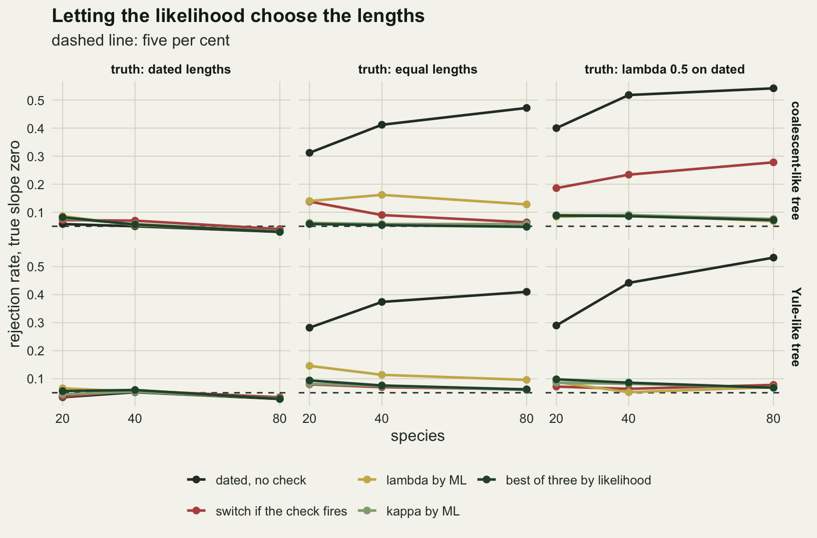
What to report
Say where the branch lengths came from: a dating analysis, a rule such as Grafen’s, or all set to one. A reader cannot judge a comparative p value without knowing whether the covariance behind it was estimated or assumed, and on the trees simulated here the choice moved the Type I error from close to nominal to 54.2 per cent in the worst cell.
Report the Garland check with its correlation and p value, for the predictor and the response, and say which lengths it was computed on. Report a check that did not fire as what it is. At 20 species on coalescent-like trees it stayed silent in more than half of the datasets that the wrong lengths turned into false positives, and on Grafen’s lengths on coalescent-like trees it fired in only 10.4 to 13.0 per cent of datasets at any size.
Do not treat the check as a verdict on the one p value in hand. In 14 of the 18 error cells it fired about as often on the undamaged datasets as on the damaged ones, so a fired check says the analysis is on the wrong tree, not that this particular slope is false, and a quiet check does not say it is true.
Fit the candidate branch length sets and report their likelihoods side by side, with lambda and kappa estimated on the dated tree as further candidates, although that combined choice was not measured here; each of the three likelihood-based repairs was measured on its own. If the slope is significant under one set and not another, that is the result to report, and the choice should be described as a choice made from the data.
Honest limits
The topology is known and correct in every dataset; only the branch lengths are wrong. Real trees have uncertain topologies, polytomies and dating error at the same time, and a topology error was not simulated.
The truth is one of three covariance models, and the analyst chooses among three sets of lengths that include two of them. Real traits need not follow any of these. An Ornstein-Uhlenbeck pull, a rate that changes across clades, or measurement error at the tips would each produce a different pattern in the Garland plot, and the good behaviour of the likelihood choice here partly reflects that the truth was usually on its list.
Both traits evolve on the same covariance. A predictor and a response that evolved on different time scales, or a response whose residual alone carries the tree, would change which diagnostic has the power, and the result that the check on the residual contrasts did no better than the predictor alone is specific to this design.
The check is the Pearson correlation at five per cent, as in Garland, Harvey and Ives (1992). Rank correlations, a log transform of the standard deviations, or a regression on node height are variants in use, and their detection rates were not measured. Grafen’s rho was fixed at one rather than estimated, and other transformations, such as Nee’s or a logarithm of the dated lengths, were not tried. Kappa was confined to the interval from zero to one, and it was estimated on the dated tree only; its success rests on the equal and dated truths being the two ends of its family, and a punctuational truth that is not exactly equal lengths, for example one with a gradual component, was not simulated.
All datasets are null. How the errors and repairs affect power against a real slope, and the width of the slope interval, was not measured, and the likelihood choice could cost power even where it keeps the Type I error close to nominal.
References
Garland T, Harvey PH, Ives AR 1992 Systematic Biology 41(1):18-32 (10.1093/sysbio/41.1.18)
Diaz-Uriarte R, Garland T 1996 Systematic Biology 45(1):27-47 (10.1093/sysbio/45.1.27)
Diaz-Uriarte R, Garland T 1998 Systematic Biology 47(4):654-672 (10.1080/106351598260653)
Grafen A 1989 Philosophical Transactions of the Royal Society B 326(1233):119-157 (10.1098/rstb.1989.0106)
Pagel M 1999 Nature 401(6756):877-884 (10.1038/44766)
Revell LJ 2010 Methods in Ecology and Evolution 1(4):319-329 (10.1111/j.2041-210X.2010.00044.x)