set.seed(20260717)
tr    <- seq(1, 7, by = 1)
traps <- as.matrix(expand.grid(x = tr, y = tr)); J <- nrow(traps)
K     <- 6
g0_true <- 0.30; sig_true <- 0.70
buffer  <- 3
xl <- range(traps[, 1]) + c(-buffer, buffer)
yl <- range(traps[, 2]) + c(-buffer, buffer)
A  <- diff(xl) * diff(yl)
N_true <- 72; D_true <- N_true / A

sx <- runif(N_true, xl[1], xl[2]); sy <- runif(N_true, yl[1], yl[2])
d2 <- outer(sx, traps[, 1], "-")^2 + outer(sy, traps[, 2], "-")^2
p  <- g0_true * exp(-d2 / (2 * sig_true^2))
yfull  <- matrix(rbinom(N_true * J, K, p), N_true, J)
caught <- rowSums(yfull) > 0
Y <- yfull[caught, , drop = FALSE]; n <- nrow(Y)
spat_recap <- sum(rowSums(Y > 0) >= 2); tot_det <- sum(Y)Bayesian spatial capture-recapture
R
capture-recapture
spatial
Bayesian
MCMC
ecology tutorial
Bayesian SCR in base R by parameter-expanded data augmentation: a from-scratch sampler for latent activity centres, and posteriors for density and abundance.
The non-spatial Bayesian capture-recapture model augments the data with pseudo-individuals and estimates how many of them really exist. It answers “how many”, but it cannot answer “how many per unit area”, because it never places the animals anywhere. Spatial capture-recapture (SCR) adds the missing ingredient: every individual, real or augmented, gets a latent activity centre with a location. Once each animal sits somewhere in a state-space, density is just the number of activity centres divided by the area, and it becomes an estimable parameter with a full posterior.
This post builds a Bayesian SCR sampler from scratch in base R using parameter-expanded data augmentation. It is the spatial companion to the non-spatial closed-population Bayesian model: the same augmentation trick for abundance, plus a Metropolis step that moves each animal’s activity centre around the state-space.
From existence to location
In the non-spatial model, augmentation attaches an inclusion indicator z_i to each of M individuals (the n detected plus M - n all-zero pseudo-individuals), and abundance is the sum of the z. That gives N, but there is nowhere for the animals to be, so density has no denominator the model can defend.
SCR keeps the inclusion indicators and adds a latent activity centre s_i for every individual, with a uniform prior over the state-space. Detection at trap j uses the half-normal encounter probability
\[p_j(s_i) = g_0 \, \exp\!\left(-\frac{\lVert s_i - x_j \rVert^2}{2\sigma^2}\right),\]
and the observed counts are \(y_{ij} \sim \text{Binomial}(K, z_i \, p_j(s_i))\). Abundance in the state-space is \(N = \sum_i z_i\) and density is \(D = N / A\). The activity centre is what turns an abundance model into a density model. Data augmentation, as Royle, Dorazio and Link (2007) showed, is equivalent to placing a discrete uniform prior on N over the integers up to M, so M must sit comfortably above the plausible abundance.
A simulated study
Same design as the frequentist post: a 7 by 7 trap grid at unit spacing, six occasions, and activity centres scattered across a buffered state-space.
Of 72 animals, 38 were detected, with 140 trap-level detections and 25 animals caught at two or more traps.
Data augmentation and the sampler
We stack the detected histories under M - n all-zero rows, fix z = 1 for detected animals, and give the augmented ones a uniform activity centre. The sampler cycles four updates: a joint Metropolis move for each activity centre (propose a small step, reject anything outside the state-space, accept on the binomial likelihood), a Gibbs update of the inclusion indicators for the augmented animals, a conjugate Beta draw for the inclusion probability, and Metropolis moves for g0 and sigma with the Jacobians for their bounded priors.
M   <- 150
Yau <- rbind(Y, matrix(0, M - n, J))
z   <- c(rep(1, n), rep(0, M - n))
s   <- matrix(0, M, 2)
for (i in 1:n) { w <- Y[i, ]; s[i, ] <- c(sum(w * traps[, 1]), sum(w * traps[, 2])) / sum(w) }
s[(n + 1):M, 1] <- runif(M - n, xl[1], xl[2])
s[(n + 1):M, 2] <- runif(M - n, yl[1], yl[2])
g0 <- 0.2; sig <- 1.0; psi <- 0.5; sig_max <- 5

pmat <- function(s, g0, sig) {
  d2 <- outer(s[, 1], traps[, 1], "-")^2 + outer(s[, 2], traps[, 2], "-")^2
  g0 * exp(-d2 / (2 * sig^2))
}
ll_ind <- function(P, z) {                         # per-individual log-likelihood
  peff <- z * P
  rowSums(matrix(dbinom(as.vector(Yau), K, as.vector(peff), log = TRUE), M, J))
}set.seed(20260717)
niter <- 8000; burn <- 3000
s_s <- 1.05; s_g0 <- 0.20; s_sig <- 0.07
keepD <- keepN <- keepg0 <- keepsig <- numeric(niter)
acc_s <- acc_g0 <- acc_sig <- 0
smean <- matrix(0, n, 2); nkeep <- 0
track <- c(which.max(rowSums(Y > 0)), order(rowSums(Y > 0))[1],
which.min(abs(rowSums(Y > 0) - 2)))
track <- unique(track)[1:3]
s_track <- vector("list", length(track))
for (t in seq_along(track)) s_track[[t]] <- matrix(NA, 0, 2)
P <- pmat(s, g0, sig)
for (it in 1:niter) {
# activity centres: joint Metropolis for all M
sp <- s + matrix(rnorm(M * 2, 0, s_s), M, 2)
inb <- sp[, 1] >= xl[1] & sp[, 1] <= xl[2] & sp[, 2] >= yl[1] & sp[, 2] <= yl[2]
Pp <- pmat(sp, g0, sig)
acc <- inb & (log(runif(M)) < (ll_ind(Pp, z) - ll_ind(P, z)))
s[acc, ] <- sp[acc, ]; P[acc, ] <- Pp[acc, ]; acc_s <- acc_s + mean(acc)
# inclusion indicators for augmented animals: Gibbs
p0 <- exp(rowSums(K * log1p(-P)))
au <- (n + 1):M
z[au] <- rbinom(M - n, 1, psi * p0[au] / (psi * p0[au] + (1 - psi)))
# inclusion probability: conjugate Beta
Nz <- sum(z); psi <- rbeta(1, 1 + Nz, 1 + M - Nz)
# g0: Metropolis on logit scale, Uniform(0,1) prior (Jacobian g0(1-g0))
lgp <- qlogis(g0) + rnorm(1, 0, s_g0); g0p <- plogis(lgp); Pg <- pmat(s, g0p, sig)
if (log(runif(1)) < sum(ll_ind(Pg, z)) + log(g0p * (1 - g0p)) -
sum(ll_ind(P, z)) - log(g0 * (1 - g0))) {
g0 <- g0p; P <- Pg; acc_g0 <- acc_g0 + 1
}
# sigma: Metropolis on log scale, Uniform(0, sig_max) prior (Jacobian sigma)
sigp <- exp(log(sig) + rnorm(1, 0, s_sig))
if (sigp < sig_max) {
Ps <- pmat(s, g0, sigp)
if (log(runif(1)) < sum(ll_ind(Ps, z)) + log(sigp) -
sum(ll_ind(P, z)) - log(sig)) {
sig <- sigp; P <- Ps; acc_sig <- acc_sig + 1
}
}
keepN[it] <- Nz; keepD[it] <- Nz / A; keepg0[it] <- g0; keepsig[it] <- sig
if (it > burn) {
nkeep <- nkeep + 1; smean <- smean + s[1:n, ]
for (t in seq_along(track)) s_track[[t]] <- rbind(s_track[[t]], s[track[t], ])
}
}
smean <- smean / nkeep; idx <- (burn + 1):niter
qD <- quantile(keepD[idx], c(.5, .025, .975))
qN <- quantile(keepN[idx], c(.5, .025, .975))
qg0 <- quantile(keepg0[idx], c(.5, .025, .975))
qs <- quantile(keepsig[idx], c(.5, .025, .975))The chain accepts activity-centre moves 0.62 of the time, and the g0 and sigma moves 0.54 and 0.46, so mixing is healthy without any tuning beyond the step sizes. The density posterior has median 0.562 animals per unit area with a 95% credible interval of [0.444, 0.708], covering the true 0.5. Abundance in the state-space has median 81 (interval [64, 102], true 72), and the posterior never approaches the augmentation ceiling of 150, so the discrete uniform prior on N is not squeezing the estimate. Detection recovers well too: g0 at 0.312 [0.243, 0.395] and sigma at 0.671 [0.603, 0.742].
arr_area <- prod(apply(traps, 2, function(z) diff(range(z))))
D_arr    <- n / arr_area
dpost <- data.frame(D = keepD[idx])
p1 <- ggplot(dpost, aes(D)) +
  geom_histogram(bins = 45, fill = forest, colour = paper, linewidth = 0.2) +
  geom_vline(xintercept = D_true, colour = ink, linewidth = 0.8) +
  geom_vline(xintercept = D_arr, colour = rust, linewidth = 0.8, linetype = "dashed") +
  annotate("text", x = D_true, y = Inf, label = "true D", vjust = 1.6, hjust = -0.1,
           colour = ink, size = 3.4) +
  annotate("text", x = D_arr, y = Inf, label = "naive: count / array", vjust = 1.6,
           hjust = 1.1, colour = rust, size = 3.4) +
  labs(x = "density (animals per unit area)", y = "posterior draws",
       title = "Density is an estimable parameter under SCR",
       subtitle = paste0("posterior median ", round(qD[1], 3),
                         ", 95% CrI [", round(qD[2], 3), ", ", round(qD[3], 3), "]")) +
  theme_te()
p1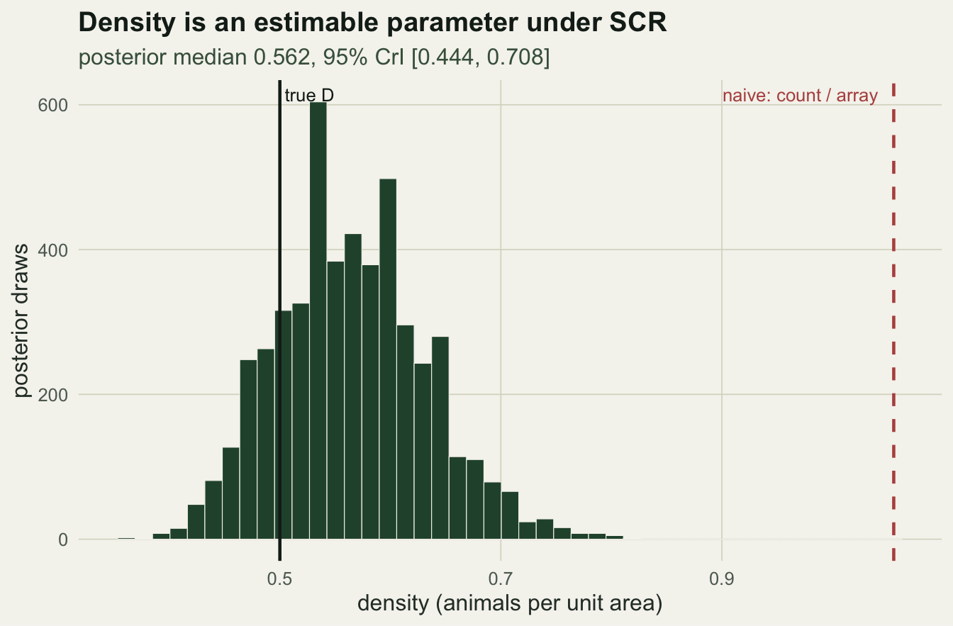
The activity centres, with their uncertainty
Because each animal’s centre is a latent variable, the sampler returns a full posterior for where it lived, not just a point. An animal caught at many traps has a sharply located centre; one caught at a single trap could sit anywhere within detection range of that trap, so its posterior is a broad cloud. Dividing the detected count by the array footprint gives 1.056 per unit area, roughly 2.1 times the truth, because that footprint ignores the animals whose centres lie off the grid but still within reach: exactly the animals SCR places explicitly.
cols <- c(forest, gold, rust)
cl <- do.call(rbind, lapply(seq_along(track), function(t) {
  data.frame(x = s_track[[t]][, 1], y = s_track[[t]][, 2],
             id = paste0(rowSums(Y > 0)[track[t]], " traps"), k = t)
}))
mn <- do.call(rbind, lapply(seq_along(track), function(t) {
  data.frame(x = mean(s_track[[t]][, 1]), y = mean(s_track[[t]][, 2]), k = t)
}))
lk <- do.call(rbind, lapply(seq_along(track), function(t) {
  js <- which(Y[track[t], ] > 0)
  data.frame(x = mn$x[t], y = mn$y[t], xe = traps[js, 1], ye = traps[js, 2], k = t)
}))
p2 <- ggplot() +
  geom_point(data = as.data.frame(traps), aes(x, y), shape = 3,
             colour = faint, size = 1.8, stroke = 0.5) +
  geom_point(data = cl, aes(x, y, colour = id), alpha = 0.05, size = 0.7) +
  geom_segment(data = lk, aes(x, y, xend = xe, yend = ye, colour = factor(k)),
               linewidth = 0.3, alpha = 0.6, show.legend = FALSE) +
  geom_point(data = cbind(mn, id = cl$id[match(mn$k, cl$k)]),
             aes(x, y, colour = id), size = 2.6) +
  scale_colour_manual(values = setNames(cols, unique(cl$id)),
                      breaks = unique(cl$id), name = "captures") +
  guides(colour = guide_legend(override.aes = list(alpha = 1, size = 2.4))) +
  coord_equal() +
  labs(x = "easting", y = "northing",
       title = "Posterior activity centres",
       subtitle = "more captures, tighter location") +
  theme_te() + theme(legend.position = "top")
p2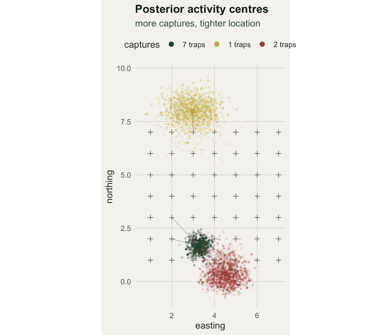
Checking the fit
A posterior-predictive check compares a feature of the observed data with the same feature in data simulated from the fitted model. The number of animals caught at two or more traps is a natural spatial summary. Simulating at the posterior medians:
set.seed(99)
obs_sr <- sum(rowSums(Y > 0) >= 2)
gm <- qg0[1]; sm <- qs[1]; Dm <- qD[1]
ppc <- replicate(1000, {
  Nsim <- rpois(1, Dm * A)
  xs <- runif(Nsim, xl[1], xl[2]); ys <- runif(Nsim, yl[1], yl[2])
  d2s <- outer(xs, traps[, 1], "-")^2 + outer(ys, traps[, 2], "-")^2
  ys2 <- matrix(rbinom(Nsim * J, K, gm * exp(-d2s / (2 * sm^2))), Nsim, J)
  cc  <- rowSums(ys2) > 0
  sum(rowSums(ys2[cc, , drop = FALSE] > 0) >= 2)
})
bp <- mean(ppc >= obs_sr)
The observed 25 spatial recaptures sit near the centre of the predictive distribution (median 28), with a Bayesian p-value of 0.74: no sign of misfit on this feature. The next posts return to design (how trap spacing controls whether sigma, and therefore density, can be pinned down) and to detection covariates with formal goodness-of-fit.
Takeaways
Non-spatial Bayesian capture-recapture gives abundance but not density, because it never locates the animals. SCR augments both existence and location: an inclusion indicator plus a latent activity centre for every individual. The sampler is a short cycle of Metropolis moves for the centres and detection parameters, a Gibbs update for inclusion, and a conjugate draw for the inclusion probability, all in base R. The reward is a full posterior for density, and a posterior for where each animal actually lived, with uncertainty that shrinks as captures accumulate.
References
Royle, J. A., Dorazio, R. M. and Link, W. A. 2007. Analysis of multinomial models with unknown index using data augmentation. Journal of Computational and Graphical Statistics 16(1):67-85 (10.1198/106186007X181425).
Royle, J. A. and Young, K. V. 2008. A hierarchical model for spatial capture-recapture data. Ecology 89(8):2281-2289 (10.1890/07-0601.1).
Royle, J. A., Karanth, K. U., Gopalaswamy, A. M. and Kumar, N. S. 2009. Bayesian inference in camera trapping studies for a class of spatial capture-recapture models. Ecology 90(11):3233-3244 (10.1890/08-1481.1).
Borchers, D. L. and Efford, M. G. 2008. Spatially explicit maximum likelihood methods for capture-recapture studies. Biometrics 64(2):377-385 (10.1111/j.1541-0420.2007.00927.x).
Royle, J. A., Chandler, R. B., Sollmann, R. and Gardner, B. 2014. Spatial Capture-Recapture. Academic Press (ISBN 978-0-12-405939-9).