---
title: "Bayesian hierarchical models with MCMC"
description: "Fit a varying-intercept Poisson model for site counts by Metropolis-within-Gibbs in base R, and see how partial pooling stabilises the data-poor sites."
date: "2026-07-14 12:00"
categories: [Bayesian statistics, MCMC, mixed models, R, ecology tutorial]
image: thumbnail.png
image-alt: "A shrinkage diagram: site count estimates move from spread-out no-pooling values toward the grand mean under partial pooling, with data-poor sites moving most."
---
The three earlier posts in this series built the pieces: a Metropolis sampler for a target with no closed form, a Gibbs sampler for conjugate updates, and the diagnostics that tell you whether a chain has converged. This post puts them together on the model that makes Bayesian computation worth the effort for ecologists, a hierarchical model with a varying intercept per site. Counts at several sites are neither all the same nor all independent, and a hierarchical model captures exactly that: it lets each site have its own rate while learning how much sites differ, so that data-poor sites borrow strength from the rest. We fit it with Metropolis steps for the parts that are not conjugate and Gibbs steps for the parts that are, then check the fit with a posterior predictive test.
```{r}
#| label: setup
#| include: false
library(ggplot2)
knitr::opts_chunk$set(echo = TRUE, message = FALSE, warning = FALSE,
fig.align = "center", dpi = 150)
paper <- "#f5f4ee"; ink <- "#16241d"; forest <- "#275139"; sage <- "#93a87f"
line_col <- "#dad9ca"; faint <- "#5d6b61"; accent2 <- "#c9b458"; warm <- "#cda23f"; brick <- "#b5534e"
theme_te <- function(base = 12) theme_minimal(base_size = base) + theme(
plot.background = element_rect(fill = paper, colour = NA),
panel.background = element_rect(fill = paper, colour = NA),
panel.grid.major = element_line(colour = line_col, linewidth = 0.3),
panel.grid.minor = element_blank(),
axis.title = element_text(colour = ink), axis.text = element_text(colour = faint),
plot.title = element_text(colour = ink, face = "bold"),
plot.subtitle = element_text(colour = faint),
legend.title = element_text(colour = ink), legend.text = element_text(colour = faint),
legend.position = "top",
strip.text = element_text(colour = ink, face = "bold"))
theme_set(theme_te())
```
## Counts at many sites, and three ways to summarise them
Suppose we count a species over several repeat visits at ten sites, with uneven effort: some sites were visited twice, others a dozen times. We want each site's mean count per visit. There are three obvious strategies. Estimate each site on its own, which is unbiased but wildly uncertain for a site seen twice. Pool everything into one number, which is stable but pretends every site is identical. Or do something in between. The data below are simulated so we know the truth: site log-rates are drawn around a common mean with real site-to-site spread.
```{r}
#| label: data
set.seed(4217)
J <- 10L
n_j <- c(2, 2, 3, 3, 4, 5, 6, 8, 10, 12)          # visits per site (uneven effort)
mu_true <- log(5); tau_true <- 0.6                 # true hyperparameters
alpha_true <- rnorm(J, mu_true, tau_true)          # true site log-rates
y <- lapply(seq_len(J), function(j) rpois(n_j[j], exp(alpha_true[j])))
S <- sapply(y, sum); ybar <- S / n_j               # site totals and mean counts
nopool <- log(pmax(ybar, 0.5))                     # each site alone (log scale)
pool   <- log(sum(S) / sum(n_j))                   # one rate for all sites
round(rbind(visits = n_j, mean_count = ybar), 2)
```
The grand mean count is `r round(sum(S) / sum(n_j), 2)` per visit, but the site means scatter from `r round(min(ybar), 1)` to `r round(max(ybar), 1)`. Some of that scatter is real difference between sites and some is just sampling noise at the thinly-visited ones. The whole job of the hierarchical model is to tell those apart.
## A varying-intercept model
Give each site its own log-rate, and tie the log-rates together with a common distribution:
$$y_{ij} \sim \text{Poisson}\!\left(e^{\alpha_j}\right), \qquad \alpha_j \sim \text{Normal}\!\left(\mu,\ \tau^2\right).$$
Here $\alpha_j$ is site $j$'s log mean count, $\mu$ is the typical log-rate across sites, and $\tau$ is the standard deviation of log-rates between sites. When $\tau$ is small the sites are nearly identical and the model pools hard; when $\tau$ is large the sites are treated as almost independent. Crucially, $\tau$ is estimated from the data, not fixed in advance, so the amount of pooling is learned. We put a flat prior on $\mu$ and the standard reference prior on $\tau^2$, exactly as in the Gibbs post.
## Metropolis within Gibbs
Now the two earlier samplers earn their keep. Conditional on the site log-rates, the hyperparameters $\mu$ and $\tau^2$ have the same conjugate full conditionals as the normal model in the Gibbs post, treating the $\alpha_j$ as the data: $\mu$ given the rest is normal, and $\tau^2$ given the rest is inverse-gamma. Those get Gibbs updates. But each $\alpha_j$ has a Poisson likelihood times a normal prior, which is not a standard distribution, so it gets a Metropolis step. Alternating conjugate Gibbs draws with Metropolis draws for the awkward coordinates is called Metropolis-within-Gibbs, and it is how most hierarchical models were fitted by hand before automatic samplers.
```{r}
#| label: sampler
# log full conditional for alpha_j (up to a constant):
#   S_j * a - n_j * exp(a) - (a - mu)^2 / (2 tau^2)
mwg <- function(n_iter, prop_sd = 0.25, init_mu = 0, init_tau2 = 1) {
  a <- rep(init_mu, J); mu <- init_mu; tau2 <- init_tau2
  A <- matrix(0, n_iter, J); MU <- numeric(n_iter); TAU2 <- numeric(n_iter); acc <- 0L
  for (t in seq_len(n_iter)) {
    for (j in seq_len(J)) {                                   # Metropolis for each alpha_j
      prop <- a[j] + rnorm(1, 0, prop_sd)
      lp_cur  <- S[j] * a[j] - n_j[j] * exp(a[j]) - (a[j] - mu)^2 / (2 * tau2)
      lp_prop <- S[j] * prop - n_j[j] * exp(prop) - (prop - mu)^2 / (2 * tau2)
      if (log(runif(1)) < lp_prop - lp_cur) { a[j] <- prop; acc <- acc + 1L }
    }
    mu   <- rnorm(1, mean(a), sqrt(tau2 / J))                 # Gibbs for mu
    tau2 <- 1 / rgamma(1, shape = J / 2, rate = sum((a - mu)^2) / 2)   # Gibbs for tau^2
    A[t, ] <- a; MU[t] <- mu; TAU2[t] <- tau2
  }
  list(A = A, mu = MU, tau2 = TAU2, acc = acc / (n_iter * J))
}

n_iter <- 20000L; burn <- 2000L; keep <- (burn + 1):n_iter
starts <- c(-1, 0.5, 2, 3.5)                                  # over-dispersed starts
set.seed(555)
chains <- lapply(starts, function(s) mwg(n_iter, prop_sd = 0.25, init_mu = s))
acc <- mean(sapply(chains, function(c) c$acc))
mu_draws  <- unlist(lapply(chains, function(c) c$mu[keep]))
tau_draws <- sqrt(unlist(lapply(chains, function(c) c$tau2[keep])))
A_draws   <- do.call(rbind, lapply(chains, function(c) c$A[keep, , drop = FALSE]))
alpha_pm  <- colMeans(A_draws)
round(c(acceptance = acc,
        mu_mean = mean(mu_draws), mu_lo = quantile(mu_draws, .025), mu_hi = quantile(mu_draws, .975),
        tau_mean = mean(tau_draws), tau_lo = quantile(tau_draws, .025), tau_hi = quantile(tau_draws, .975)), 3)
```
The Metropolis steps accept about `r round(acc * 100)` per cent of proposals. The hyperparameters land where they should: the posterior mean of $\mu$ is `r round(mean(mu_draws), 2)` against a true `r round(mu_true, 2)`, and the posterior mean of the between-site standard deviation $\tau$ is `r round(mean(tau_draws), 2)` against a true `r round(tau_true, 2)`, with a 95 per cent interval of `r round(quantile(tau_draws, .025), 2)` to `r round(quantile(tau_draws, .975), 2)` that comfortably includes it.
## Checking convergence
Four dispersed chains let us apply the split R-hat from the diagnostics post to every parameter, not just the ones we happen to care about. A hierarchical model has many parameters that must all converge together, and it is easy for the variance $\tau^2$ to mix poorly even when the means look fine.
```{r}
#| label: rhat
rhat_split <- function(mat) {                 # mat: iterations x chains
  n <- nrow(mat); half <- n %/% 2
  sp <- cbind(mat[1:half, , drop = FALSE], mat[(n - half + 1):n, , drop = FALSE]); n2 <- half
  cm <- colMeans(sp); cv <- apply(sp, 2, var); W <- mean(cv); B <- n2 * var(cm)
  sqrt((((n2 - 1) / n2) * W + B / n2) / W)
}
rhat_mu    <- rhat_split(sapply(chains, function(c) c$mu[keep]))
rhat_tau   <- rhat_split(sapply(chains, function(c) sqrt(c$tau2[keep])))
rhat_alpha <- sapply(seq_len(J), function(j) rhat_split(sapply(chains, function(c) c$A[keep, j])))
round(c(rhat_mu = rhat_mu, rhat_tau = rhat_tau, rhat_alpha_max = max(rhat_alpha)), 3)
```
Every R-hat is at or below `r round(max(c(rhat_mu, rhat_tau, max(rhat_alpha))), 3)`, well under the `1.01` threshold, so the sampler has converged on all fronts. Only now is it safe to read the results.
## Partial pooling in action
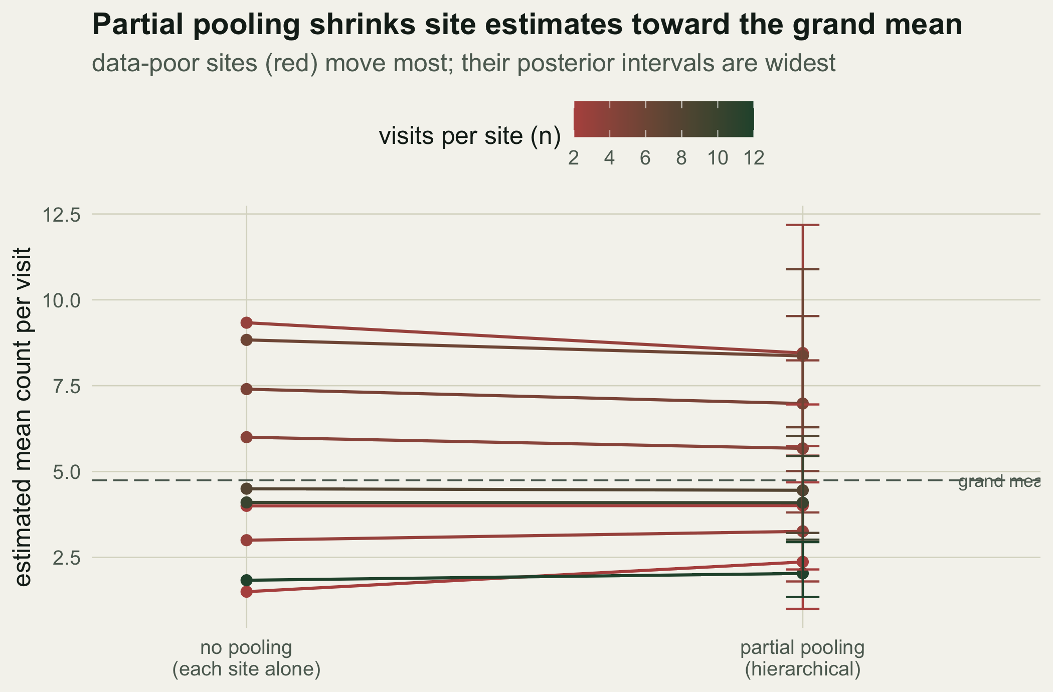
The point of the model is what it does to the site estimates. Compare each site's own estimate, the mean of its counts, with its posterior mean under the hierarchical model. The hierarchical estimates are pulled toward the grand mean, and the pull is strongest where the site's own data are weakest.
```{r}
#| label: fig-shrinkage
#| fig-cap: "Site mean-count estimates under no pooling and under partial pooling, connected per site and coloured by number of visits. Data-poor sites (red) shrink most toward the grand mean (dashed), and their posterior intervals are widest."
#| fig-alt: "Two columns of points joined by lines. The left no-pooling column is spread from about 1.5 to 9; the right partial-pooling column is more clustered around the grand mean. Red lines, for sites with few visits, move the most."
#| fig-width: 7
#| fig-height: 4.6
grand <- exp(pool); nopool_c <- exp(nopool); partial_c <- exp(alpha_pm)
ci <- t(apply(A_draws, 2, function(col) exp(quantile(col, c(0.025, 0.975)))))
seg <- data.frame(site = factor(seq_len(J)), n = n_j, nopool = nopool_c, partial = partial_c,
                  lo = ci[, 1], hi = ci[, 2])
long <- rbind(data.frame(site = seg$site, n = seg$n, x = 1, y = seg$nopool),
              data.frame(site = seg$site, n = seg$n, x = 2, y = seg$partial))
ggplot() +
  geom_hline(yintercept = grand, colour = faint, linetype = "longdash", linewidth = 0.4) +
  geom_line(data = long, aes(x, y, group = site, colour = n), linewidth = 0.7) +
  geom_point(data = long, aes(x, y, colour = n), size = 2) +
  geom_errorbar(data = seg, aes(x = 2, ymin = lo, ymax = hi, colour = n), width = 0.06, linewidth = 0.5) +
  scale_colour_gradient(low = brick, high = forest, name = "visits per site (n)") +
  scale_x_continuous(breaks = c(1, 2),
                     labels = c("no pooling\n(each site alone)", "partial pooling\n(hierarchical)"),
                     limits = c(0.8, 2.35)) +
  annotate("text", x = 2.28, y = grand, label = "grand mean", hjust = 0, colour = faint, size = 3) +
  labs(x = NULL, y = "estimated mean count per visit",
       title = "Partial pooling shrinks site estimates toward the grand mean",
       subtitle = "data-poor sites (red) move most; their posterior intervals are widest")
```
```{r}
#| label: shrinkage-numbers
poor <- 2L    # a site visited only twice, with two low counts
rich <- 10L   # a well-sampled site with a similarly low raw mean
round(c(poor_visits = n_j[poor], poor_raw = exp(nopool[poor]), poor_partial = exp(alpha_pm[poor]),
        rich_visits = n_j[rich], rich_raw = exp(nopool[rich]), rich_partial = exp(alpha_pm[rich])), 2)
```
Two sites make the mechanism concrete. One site was visited only twice and happened to record low counts, giving a raw mean of `r round(exp(nopool[poor]), 1)`; the model pulls its estimate up to `r round(exp(alpha_pm[poor]), 1)`, a long way toward the grand mean of `r round(grand, 1)`, because two visits carry little weight against the population of sites. Another site with a similarly low raw mean of `r round(exp(nopool[rich]), 1)` was visited twelve times; the model barely moves it, to `r round(exp(alpha_pm[rich]), 1)`, because its data are strong enough to stand on their own. That is partial pooling: the shrinkage is not uniform but proportional to how little each site knows, which is exactly the behaviour a frequentist mixed model produces through its random effects.
## Does the model fit? A posterior predictive check
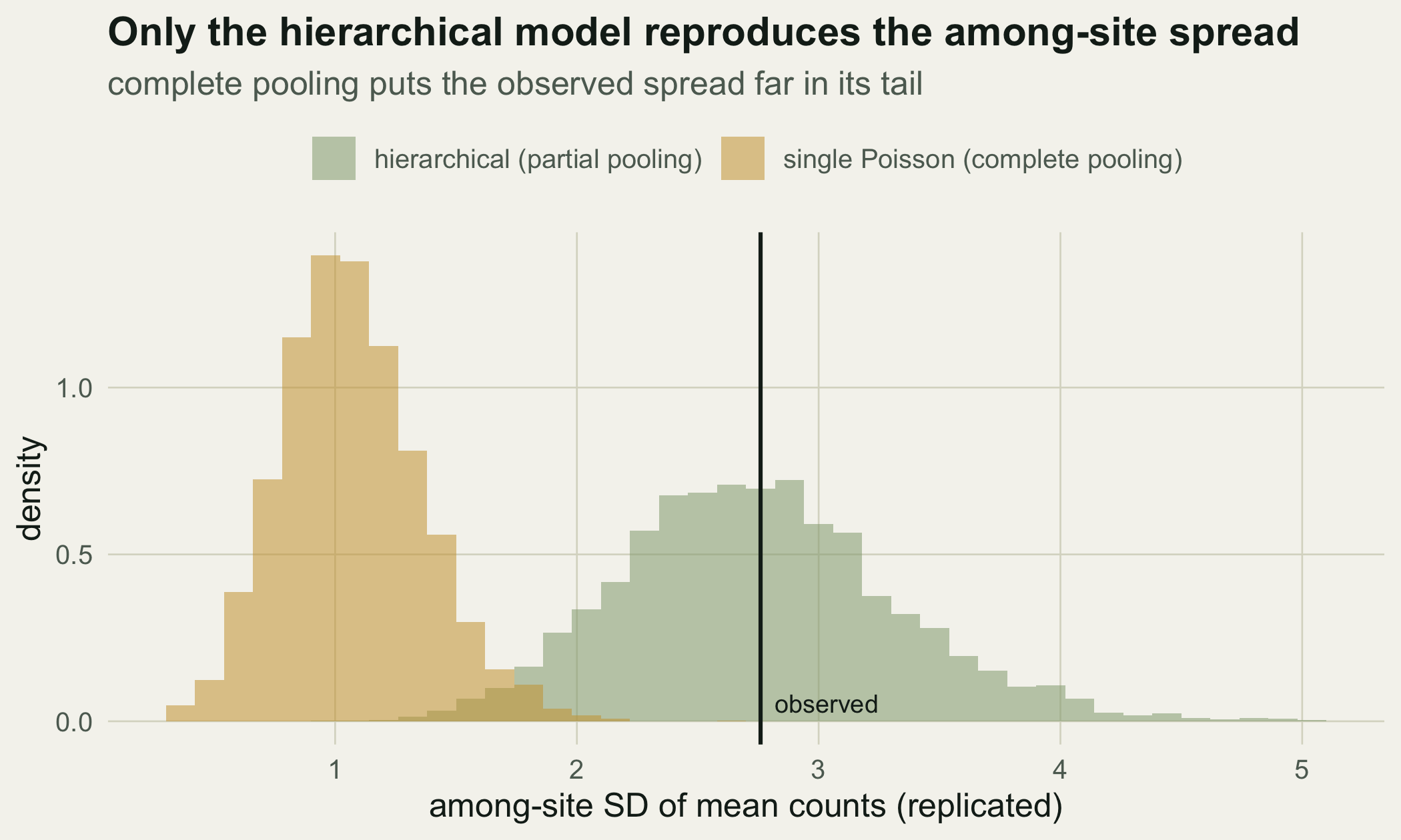
Recovering the parameters is not the same as fitting the data. A posterior predictive check simulates fresh datasets from the fitted model and asks whether they look like what we observed, on a statistic the model was not directly fitted to. A natural choice here is the spread of mean counts across sites, since capturing among-site variation is the whole reason to go hierarchical. We compare the hierarchical model against the complete-pooling alternative, a single Poisson with one rate.
```{r}
#| label: ppc
T_obs <- sd(ybar)                                           # observed among-site spread
set.seed(88)                                                # hierarchical replicates
idx <- sample(nrow(A_draws), 4000)
T_hier <- sapply(idx, function(i) {
  a <- A_draws[i, ]
  sd(sapply(seq_len(J), function(j) mean(rpois(n_j[j], exp(a[j])))))
})
set.seed(89)                                                # complete-pooling replicates
lam_draws <- rgamma(4000, shape = sum(S) + 0.001, rate = sum(n_j) + 0.001)
T_pool <- sapply(lam_draws, function(lam)
  sd(sapply(seq_len(J), function(j) mean(rpois(n_j[j], lam)))))
round(c(observed = T_obs, hier_mean = mean(T_hier), hier_p = mean(T_hier >= T_obs),
        pool_mean = mean(T_pool), pool_p = mean(T_pool >= T_obs)), 3)
```
The observed among-site standard deviation is `r round(T_obs, 2)`. Datasets simulated from the hierarchical model have a spread averaging `r round(mean(T_hier), 2)`, right on top of it, and the observed value falls near the middle of the replicate distribution with a Bayesian p-value of `r round(mean(T_hier >= T_obs), 2)`: the model reproduces the variation it was built to capture. The single-Poisson model is a different story. Its replicates spread only `r round(mean(T_pool), 2)` on average, because a single rate allows no real site-to-site variation, and the observed value sits far out in its tail with a Bayesian p-value of `r round(mean(T_pool >= T_obs), 3)`. Complete pooling is decisively rejected for underdispersion.
```{r}
#| label: fig-ppc
#| fig-cap: "Posterior predictive distributions of the among-site spread. The hierarchical model (green) brackets the observed value; the single-Poisson model (gold) falls well short, placing the observation in its extreme tail."
#| fig-alt: "Two overlaid histograms of a replicated spread statistic. The green hierarchical distribution is centred on the observed vertical line; the gold complete-pooling distribution sits to its left, with the observed line in its far right tail."
#| fig-width: 7
#| fig-height: 4.2
ppc <- rbind(data.frame(T = T_hier, model = "hierarchical (partial pooling)"),
             data.frame(T = T_pool, model = "single Poisson (complete pooling)"))
ppc$model <- factor(ppc$model, levels = c("hierarchical (partial pooling)",
                                          "single Poisson (complete pooling)"))
ggplot(ppc, aes(T, fill = model)) +
  geom_histogram(aes(y = after_stat(density)), binwidth = 0.12, colour = NA, alpha = 0.55,
                 position = "identity") +
  geom_vline(xintercept = T_obs, colour = ink, linewidth = 0.7) +
  annotate("text", x = T_obs, y = 0, label = "  observed", hjust = 0, vjust = -0.5, colour = ink, size = 3.2) +
  scale_fill_manual(values = c("hierarchical (partial pooling)" = sage,
                               "single Poisson (complete pooling)" = warm), name = NULL) +
  labs(x = "among-site SD of mean counts (replicated)", y = "density",
       title = "Only the hierarchical model reproduces the among-site spread",
       subtitle = "complete pooling puts the observed spread far in its tail")
```
## Where this leaves you
This one model uses everything the series built. The site rates needed Metropolis steps because their conditionals are not standard; the hyperparameters used Gibbs steps because theirs are; the whole thing was trusted only after R-hat confirmed convergence across every parameter; and the fit was judged by a posterior predictive check rather than by parameter recovery alone. The reward is partial pooling, which gives stable estimates for data-poor sites without erasing the real differences between them, and honest uncertainty for each one. A frequentist mixed model reaches similar point estimates by a faster route, but coding the sampler by hand shows exactly where the pooling comes from and makes it straightforward to extend, to site-level covariates, non-normal group effects, or several grouping factors at once, none of which change the basic recipe.
## Related tutorials
- [Metropolis-Hastings from scratch](../metropolis-hastings-from-scratch/)
- [Gibbs sampling with conjugate updates](../gibbs-sampling-conjugate/)
- [Marginal and conditional R-squared](../marginal-vs-conditional-r2/)
- [Choosing priors: flat is not uninformative](../choosing-priors-flat-not-uninformative/)
## References
- Gelfand AE, Hills SE, Racine-Poon A, Smith AFM 1990 Journal of the American Statistical Association 85(412):972-985 (10.1080/01621459.1990.10474968)
- Gelman A, Meng XL, Stern H 1996 Statistica Sinica 6(4):733-807 (ISSN 1017-0405)
- Kery M, Royle JA 2016 Applied Hierarchical Modeling in Ecology, Volume 1 (ISBN 978-0-12-801378-6)
- Gelman A, Hill J 2007 Data Analysis Using Regression and Multilevel/Hierarchical Models (ISBN 978-0-521-68689-1)
- Gelman A, Carlin JB, Stern HS, Dunson DB, Vehtari A, Rubin DB 2013 Bayesian Data Analysis, 3rd edition (ISBN 978-1-4398-4095-5)