Bayesian closed capture-recapture

Estimate closed-population size in R with parameter-expanded data augmentation: inclusion indicators, conjugate Gibbs updates, and a posterior for the animals never seen.

Trap a closed population over several occasions and count the distinct animals caught. That count is a lower bound on population size, never the size itself, because some animals are never caught at all. The whole problem is estimating how many you missed, and the elegant Bayesian answer is to invent a pool of animals that might exist and let the data decide which of them are real. That is parameter-expanded data augmentation, and it is the cleanest example of the idea running through this series: put the unknown in the sampler.

The frequentist treatment writes down a likelihood for the number seen and profiles out population size. Here the unknown size itself becomes a sum of latent inclusion indicators, and the sampler is three conjugate updates.

The model

Under model M0, every animal is caught on each of K occasions with the same probability p, independently. We never observe the animals caught zero times, so the data are the capture histories of the n distinct animals seen.

Augmentation handles the unknown size like this. Take the n observed histories and pad the data set with all-zero histories up to a large ceiling M, comfortably above any plausible population size. Each of the M pseudo-animals gets an inclusion indicator: a Bernoulli draw with probability omega that says whether it is a real member of the population. True population size is the number of ones. An animal that is included is caught with probability p; one that is not included is never caught. The observed animals are certainly included; the padded zeros are the question mark, and their inclusion probability given a zero history is what the sampler resolves.

Simulating and augmenting

set.seed(1873)
N.true <- 300L; K <- 6L; p.true <- 0.30
Y.full <- matrix(rbinom(N.true * K, 1, p.true), N.true, K)   # every animal
detected <- rowSums(Y.full) > 0
Yobs <- Y.full[detected, , drop = FALSE]                     # only the seen ones
nobs <- nrow(Yobs); never.true <- N.true - nobs

The naive estimate is the number of distinct animals seen.

naive.N <- nobs

Here 259 animals are seen, and 41 are never caught. Now augment: pad with all-zero histories up to a ceiling.

M <- 600L                                        # augmentation ceiling
Yaug <- rbind(Yobs, matrix(0L, M - nobs, K))
ysum <- rowSums(Yaug)                             # capture frequency per pseudo-animal
zero <- ysum == 0

A Gibbs sampler over inclusion

Each sweep updates three things. Inclusion probability omega is a conjugate Beta given how many pseudo-animals are currently included. Detection p is a conjugate Beta over the captures of the included animals. Then each zero-history pseudo-animal draws a new inclusion indicator, whose probability weighs “included but never caught”, proportional to omega times the chance of six misses, against “not a member”. Observed animals stay included.

n.iter <- 12000L; burn <- 2000L
N.s <- numeric(n.iter); p.s <- numeric(n.iter)
z <- as.integer(ysum > 0); omega <- 0.5; pp <- 0.5
for (it in 1:n.iter) {
  sz <- sum(z)
  # inclusion probability: conjugate Beta
  omega <- rbeta(1, 1 + sz, 1 + M - sz)
  # detection over included animals: conjugate Beta
  succ <- sum(ysum[z == 1]); opp <- sz * K
  pp <- rbeta(1, 1 + succ, 1 + opp - succ)
  # inclusion indicators for zero-history pseudo-animals
  psi <- omega * (1 - pp)^K / (omega * (1 - pp)^K + (1 - omega))
  z[zero] <- rbinom(sum(zero), 1, psi)
  z[!zero] <- 1L
  N.s[it] <- sum(z); p.s[it] <- pp
}
keep <- (burn + 1):n.iter
N.post <- N.s[keep]; p.post <- p.s[keep]; unseen.post <- N.post - nobs

Population size is the derived quantity sum(z), so its posterior comes free from the inclusion indicators. No profile likelihood, no delta-method interval: the uncertainty in how many animals were missed is represented directly.

What the posterior recovers

N.med <- median(N.post); N.ci <- quantile(N.post, c(.025, .975))
p.med <- median(p.post); p.ci <- quantile(p.post, c(.025, .975))
un.med <- median(unseen.post); un.ci <- quantile(unseen.post, c(.025, .975))

Population size has posterior median 290 with a 95% credible interval of [278, 306], covering the true 300, while the naive count of 259 sits well below the lower end. Detection lands at 0.311 [0.284, 0.337], close to 0.30. The posterior probability that the population exceeds the number actually seen is 1, which is only sensible: you cannot have seen more animals than exist.

library(ggplot2)
ink <- "#16241d"; forest <- "#275139"; sage <- "#93a87f"; paper <- "#f5f4ee"
rust <- "#b5534e"; gold <- "#cda23f"; line <- "#dad9ca"
theme_te <- theme_minimal(base_size = 12) +
  theme(panel.grid.minor = element_blank(),
        panel.grid.major = element_line(colour = line, linewidth = 0.3),
        plot.title = element_text(colour = ink, face = "bold", size = 13),
        plot.subtitle = element_text(colour = "#5d6b61", size = 10),
        axis.title = element_text(colour = ink), axis.text = element_text(colour = "#46604a"),
        legend.position = "none")
ggplot(data.frame(N = N.post), aes(N)) +
  geom_histogram(aes(y = after_stat(density)), bins = 40, fill = sage, colour = paper, linewidth = 0.15) +
  geom_vline(xintercept = N.true, colour = rust, linewidth = 0.8) +
  geom_vline(xintercept = naive.N, colour = gold, linewidth = 0.8, linetype = "dashed") +
  labs(title = "Posterior population size from augmented capture histories",
       subtitle = "Red: true N. Gold dashed: naive count of distinct animals seen.",
       x = "Population size N", y = "Posterior density") + theme_te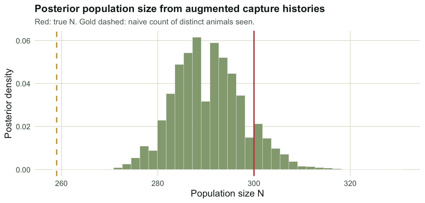

Figure 1: Posterior population size against the truth and the naive count of animals seen.

Estimating the animals no one saw

The augmentation gives a posterior for the zero-capture class directly: how many animals were present but never caught. Placed next to the observed capture frequencies, it fills in the one bar the data cannot show.

obs.freq <- tabulate(rowSums(Yobs), K)
un.mean <- mean(unseen.post); un.lo <- quantile(unseen.post, .025); un.hi <- quantile(unseen.post, .975)
df2 <- data.frame(times = 0:K, count = c(un.mean, obs.freq),
                  lo = c(un.lo, obs.freq), hi = c(un.hi, obs.freq),
                  kind = c("estimated", rep("observed", K)))
ggplot(df2, aes(times, count, fill = kind)) +
  geom_col(width = 0.7) +
  geom_errorbar(data = subset(df2, kind == "estimated"),
                aes(ymin = lo, ymax = hi), width = 0.25, colour = ink, linewidth = 0.5) +
  geom_point(aes(x = 0, y = never.true), colour = rust, size = 2.5) +
  scale_fill_manual(values = c(estimated = gold, observed = forest)) +
  scale_x_continuous(breaks = 0:K) +
  labs(title = "Capture frequency, with the estimated never-seen class",
       subtitle = "Green: animals seen 1 to K times. Gold: posterior for the zero class. Red: truth.",
       x = "Times captured", y = "Number of animals") + theme_te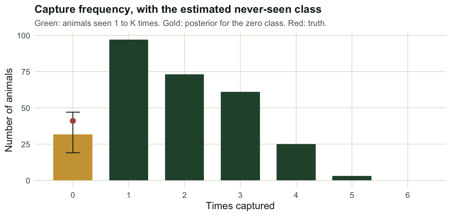

Figure 2: Observed capture frequencies with the posterior for the never-seen class.

The estimated never-seen count has posterior median 31 [19, 47], bracketing the true 41. The median runs a little low, which is the mild negative bias closed-population estimators carry when detection is imperfect, but the interval is honest about how many animals could be hiding.

A caution and a caveat

Two things to watch. The ceiling M must sit well above the posterior mass, or it truncates the estimate; check that the largest sampled size is comfortably under M and raise it if not. And constant detection is a strong assumption: if some animals are inherently harder to catch, the missed ones are the hardest of all, and population size becomes weakly identified. That heterogeneity problem is the classic warning of the closed-population literature, and no amount of data fully resolves it, so it is a modelling choice to defend rather than a detail to ignore.

Closing the series

This is the last of four Bayesian latent-state tutorials, and they are all the same move with a different hidden quantity. In survival the latent state is whether a marked animal is still alive; in abundance it is how many animals a site holds; in movement it is the true path behind noisy fixes; and here it is whether an augmented animal exists at all. In every case a naive summary of the observations, the return rate, the maximum count, the raw track, the tally of animals seen, points the wrong way, and in every case putting the unobserved quantity into the sampler and giving the observations their detection model recovers the truth with honest uncertainty. Conjugacy or a small filter handles the parameters. What changes from problem to problem is only the latent variable; the pattern is fixed.

References

• Otis, Burnham, White, Anderson 1978, Wildlife Monographs 62:3-135 (10.2307/3830650)
• Royle, Dorazio 2008, Hierarchical Modeling and Inference in Ecology, ISBN 978-0-12-374097-7
• Royle, Dorazio 2012, Journal of Ornithology 152:521-537 (10.1007/s10336-010-0619-4)
• Tanner, Wong 1987, Journal of the American Statistical Association 82(398):528-540 (10.1080/01621459.1987.10478458)
• Kery, Schaub 2012, Bayesian Population Analysis using WinBUGS, ISBN 978-0-12-387020-9

Related tutorials

• Closed-population capture-recapture
• Bayesian N-mixture abundance
• Bayesian state-space movement
• Bayesian spatial capture-recapture