set.seed(4816)
n.occ <- 6
marked <- rep(30, n.occ - 1)          # 30 newly marked at occasions 1..5
phi.true <- 0.72
p.true <- 0.42
N <- sum(marked)                       # total marked

CH <- matrix(0, N, n.occ)              # capture histories
f <- integer(N)                        # first-capture (marking) occasion
row <- 0
for (g in seq_along(marked)) for (k in seq_len(marked[g])) {
  row <- row + 1
  f[row] <- g
  CH[row, g] <- 1                      # marked and released
  alive <- TRUE
  for (t in (g + 1):n.occ) {
    if (alive) alive <- (runif(1) < phi.true)
    if (alive && runif(1) < p.true) CH[row, t] <- 1
  }
}
last <- apply(CH, 1, function(x) max(which(x == 1)))Bayesian Cormack-Jolly-Seber survival
Bayesian statistics
MCMC
survival analysis
R
ecology tutorial
Fit an open-population Cormack-Jolly-Seber survival model by hand in R: latent alive-state data augmentation, conjugate Gibbs updates, and honest credible intervals.
When you mark animals and resight them over several occasions, the quantity you want is apparent survival: the probability that a marked animal is alive and available on the next occasion. The trap is that an animal seen at occasion 3 and never again might have died, or might simply have gone undetected. The raw return rate, the fraction of marked animals ever seen again, folds survival and detection into one number and lands below the truth.
The Cormack-Jolly-Seber (CJS) model separates the two. Its frequentist form, a multinomial likelihood over the m-array of releases and first recaptures, is covered elsewhere on the blog. Here we fit the same model the Bayesian way, and the machinery is instructive: the alive-or-dead status of each animal after its last sighting is a latent variable, and we sample it explicitly. That is data augmentation, and it turns an awkward marginal likelihood into two conjugate updates.
The model
Each individual i is first captured (marked) at occasion f_i. After that it carries a latent alive-state z that follows a two-state chain with death absorbing:
- survival:
zat occasiontis Bernoulli with probabilityphiif the animal was alive att-1, and zero once dead; - observation: an alive animal is seen with recapture probability
p, a dead one never.
We place flat Beta(1, 1) priors on both phi and p. Because death is absorbing, the entire latent history of an animal reduces to a single number: the last occasion on which it is alive. Call it d_i. An animal last seen at occasion l_i is certainly alive up to l_i, so d_i ranges over l_i to the final occasion, with the final value meaning it survived the whole study.
Simulating a capture history
We mark 30 new animals at each of the first five occasions and follow them over six, with constant survival 0.72 and recapture 0.42.
The naive apparent return rate is the fraction of marked animals seen again at least once after release.
ever.recap <- sapply(1:N, function(i) any(CH[i, (f[i] + 1):n.occ] == 1))
naive.return <- mean(ever.recap)
That comes to 0.407, and 89 of the 150 animals are never re-encountered. Some of those are dead; many are simply alive and unseen. The return rate cannot tell them apart, so it underestimates survival.
A Gibbs sampler with the latent time of death
Each sweep does two things. First, for every animal, draw its latent last-alive occasion d_i from its full conditional. An animal last seen at l_i survives to occasion t with probability phi per step, stays unseen over those steps with probability 1 - p per step, and either dies afterwards (a factor 1 - phi when t is before the end) or survives the study. That gives an unnormalised probability over the candidate occasions, which we sample directly:
n.iter <- 15000L
burn <- 3000L
phi.s <- numeric(n.iter); p.s <- numeric(n.iter)
nalive <- matrix(0L, n.iter, n.occ)

phi <- 0.5; p <- 0.5; d <- last
for (it in 1:n.iter) {
  # draw latent last-alive occasion for each animal
  for (i in 1:N) {
    li <- last[i]
    if (li == n.occ) { d[i] <- n.occ; next }
    ts <- li:n.occ
    steps <- ts - li
    logw <- steps * log(phi) + steps * log(1 - p) +
            ifelse(ts < n.occ, log(1 - phi), 0)
    w <- exp(logw - max(logw))
    d[i] <- sample(ts, 1, prob = w)
  }
  # conjugate survival update: successes and one death per animal that dies
  phi <- rbeta(1, 1 + sum(d - f), 1 + sum(d < n.occ))
  # conjugate recapture update over alive, post-release occasions
  opp <- 0L; rec <- 0L
  for (i in 1:N) if (d[i] > f[i]) {
    idx <- (f[i] + 1):d[i]
    opp <- opp + length(idx)
    rec <- rec + sum(CH[i, idx])
  }
  p <- rbeta(1, 1 + rec, 1 + opp - rec)
  phi.s[it] <- phi; p.s[it] <- p
  for (t in 1:n.occ) nalive[it, t] <- sum(f <= t & d >= t)
}
keep <- (burn + 1):n.iter
phi.post <- phi.s[keep]; p.post <- p.s[keep]
Given the sampled trajectories, both parameters have conjugate Beta full conditionals. Survival counts the surviving steps against the deaths; recapture counts sightings against opportunities, but only on the occasions where an animal is inferred to be alive. No optimiser and no marginal likelihood: the latent states do the work.
What the posterior recovers
phi.med <- median(phi.post); phi.ci <- quantile(phi.post, c(.025, .975))
p.med <- median(p.post); p.ci <- quantile(p.post, c(.025, .975))
Survival has posterior median 0.685 with a 95% credible interval of [0.586, 0.79], covering the true 0.72. Recapture lands at 0.397 [0.297, 0.511], close to 0.42. The naive return rate of 0.407 sits below the lower end of the survival interval, so the data rule it out as a survival estimate: the posterior probability that survival exceeds the return rate is 1.
library(ggplot2); library(dplyr)
ink <- "#16241d"; forest <- "#275139"; rust <- "#b5534e"; gold <- "#cda23f"; line <- "#dad9ca"
theme_te <- theme_minimal(base_size = 12) +
  theme(panel.grid.minor = element_blank(),
        panel.grid.major = element_line(colour = line, linewidth = 0.3),
        plot.title = element_text(colour = ink, face = "bold", size = 13),
        plot.subtitle = element_text(colour = "#5d6b61", size = 10),
        axis.title = element_text(colour = ink), axis.text = element_text(colour = "#46604a"),
        strip.text = element_text(colour = ink, face = "bold"), legend.position = "none")

d1 <- bind_rows(
  data.frame(param = "Apparent survival (phi)", value = phi.post),
  data.frame(param = "Recapture probability (p)", value = p.post))
truth <- data.frame(param = c("Apparent survival (phi)", "Recapture probability (p)"),
                    x = c(phi.true, p.true))
naive.df <- data.frame(param = "Apparent survival (phi)", x = naive.return)
ggplot(d1, aes(value)) +
  geom_density(fill = forest, colour = forest, alpha = 0.35, linewidth = 0.5) +
  geom_vline(data = truth, aes(xintercept = x), colour = rust, linewidth = 0.7) +
  geom_vline(data = naive.df, aes(xintercept = x), colour = gold, linewidth = 0.7, linetype = "dashed") +
  facet_wrap(~param, scales = "free") +
  labs(title = "Posterior survival and recapture, with the naive return rate",
       subtitle = "Red: simulating truth. Gold dashed: naive apparent return rate (survival panel).",
       x = "Value", y = "Posterior density") +
  theme_te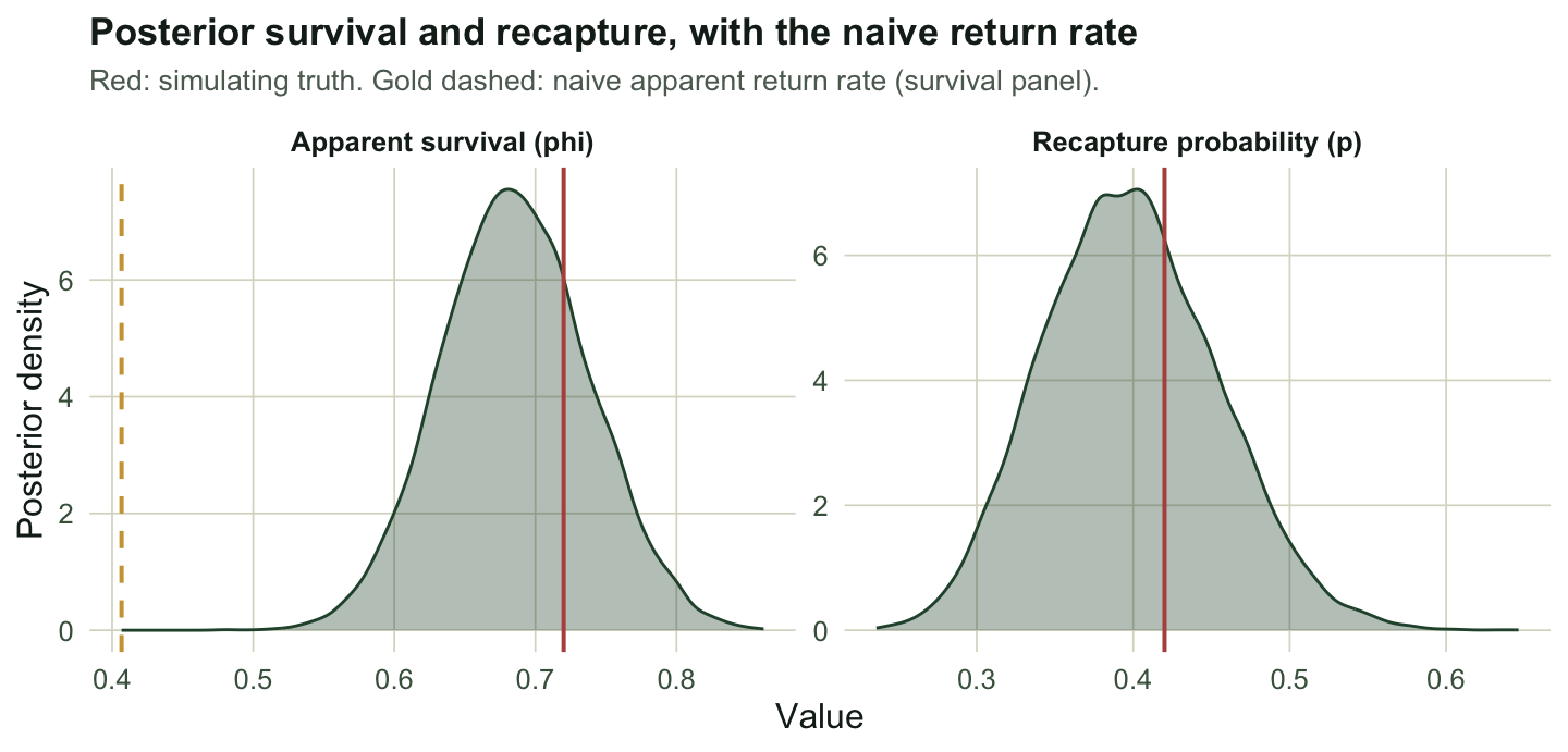
Seeing the augmentation at work
The reason the estimate beats the return rate is that the sampler carries alive-but-unseen animals in every draw. Summing the latent alive-states by occasion gives a posterior count of animals present, which always sits above the number actually detected.
library(tidyr)
sage <- "#93a87f"
n.det <- colSums(CH)
al.mean <- colMeans(nalive[keep, ])
al.lo <- apply(nalive[keep, ], 2, quantile, 0.025)
al.hi <- apply(nalive[keep, ], 2, quantile, 0.975)
d2 <- data.frame(occ = 1:n.occ, det = n.det, mean = al.mean, lo = al.lo, hi = al.hi)
ggplot(d2, aes(occ)) +
  geom_ribbon(aes(ymin = lo, ymax = hi), fill = sage, alpha = 0.35) +
  geom_line(aes(y = mean), colour = forest, linewidth = 0.8) +
  geom_point(aes(y = mean), colour = forest, size = 2) +
  geom_col(aes(y = det), fill = ink, width = 0.18) +
  scale_x_continuous(breaks = 1:n.occ) +
  labs(title = "Latent alive individuals versus detections per occasion",
       subtitle = "Bars: individuals detected. Line and band: posterior alive count.",
       x = "Occasion", y = "Number of individuals") +
  theme_te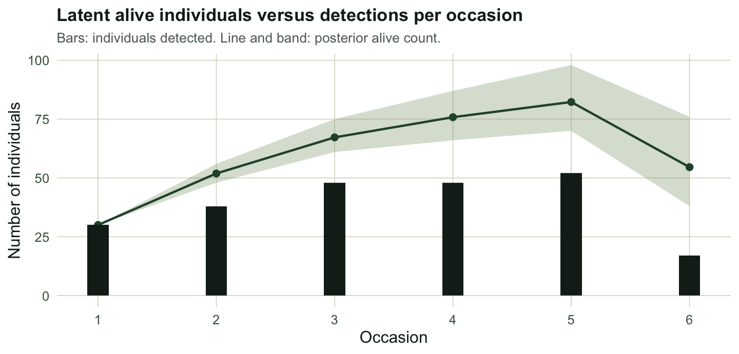
At the final occasion only 17 animals are detected, yet the posterior puts about 55 alive. Those unseen survivors are exactly what the return rate throws away and what the latent-state model keeps.
Where this sits
The recipe generalises. Any capture-recapture or occupancy model with a partially observed state can be written this way: put the latent state in the sampler, give the observed data its detection model, and let conjugacy or a small Metropolis step handle the parameters. The same augmentation drives the Bayesian occupancy model, where the latent state is site occupancy rather than individual survival, and the closed-population version, where the unknown itself is how many animals exist. What changes is the latent variable; the pattern does not.
One practical note: the latent-state sweep induces autocorrelation in the chains, so run long and check the effective sample size rather than trusting the raw draw count. Here 12,000 post-warmup draws give stable intervals, but a harder data set may need more.
References
- Cormack 1964, Biometrika 51(3-4):429-438 (10.1093/biomet/51.3-4.429)
- Jolly 1965, Biometrika 52(1-2):225-247 (10.1093/biomet/52.1-2.225)
- Seber 1965, Biometrika 52(1-2):249-259 (10.2307/2333827)
- Lebreton, Burnham, Clobert, Anderson 1992, Ecological Monographs 62(1):67-118 (10.2307/2937171)
- Royle 2008, Biometrics 64(2):364-370 (10.1111/j.1541-0420.2007.00891.x)
- King 2012, Interface Focus 2(2):190-204 (10.1098/rsfs.2011.0078)
- Kery, Schaub 2012, Bayesian Population Analysis using WinBUGS, ISBN 978-0-12-387020-9