---
title: "Variation partitioning in R: how much do environment and space each explain?"
description: "When your predictors overlap, a single R-squared double-counts shared structure. Use varpart() in R to split community variation into pure environment, pure space, and the spatially structured fraction, then test the pieces with partial RDA."
date: "2026-06-21 15:00"
categories: [Multivariate, Ordination, vegan]
image: thumbnail.png
image-alt: "A two-circle Venn diagram partitioning community variation into environment-only, space-only, and shared fractions."
---
The [constrained ordination tutorial](../constrained-ordination-dbrda/) ended with a single number: the predictors explained roughly half the variation in community composition. That number is useful, but it hides a question you usually care about. Suppose you have two *kinds* of predictors, say measured environment and geographic position. How much does each explain on its own, and how much do they explain jointly because they are correlated? A plain adjusted R-squared cannot tell you, because it lumps everything together.
This matters most when environment is spatially structured, which it almost always is. Soil moisture, temperature, and nutrients vary smoothly across a landscape, so "environment explains 40%" silently includes a chunk of pure spatial pattern. If you also fit space and get 35%, you cannot add them: the two overlap. Variation partitioning, introduced by Borcard, Legendre and Drapeau (1992), pulls the overlap apart into named fractions you can interpret and, for some of them, test.
## The setup: environment that is partly spatial
The teaching landscape has 60 plots scattered across a unit square. Two environmental variables are measured. Moisture tracks an east-west gradient, so it is spatially structured. Nutrients vary at random across the map, with no spatial pattern at all. On top of that, the community responds to a third driver: a north-south field that we did *not* measure, standing in for dispersal or some unrecorded gradient. That hidden driver is spatially structured too, so a trend surface of the coordinates can pick it up even though no environmental column does.
```{r}
#| label: data
#| message: false
#| warning: false
library(vegan)
library(ggplot2)

set.seed(71)

n <- 60
x <- runif(n)
y <- runif(n)

# moisture tracks the east-west gradient (spatially structured)
# nutrients are random across the map (no spatial signal)
moisture  <- as.numeric(scale(x)) + rnorm(n, 0, 0.35)
nutrients <- rnorm(n)

# an unmeasured, spatially structured driver of the community (north-south)
sfield <- as.numeric(scale(y))

# 20 species respond to all three with random coefficients
n_sp    <- 20
b_moist <- rnorm(n_sp, 0, 0.62)
b_nutr  <- rnorm(n_sp, 0, 0.42)
b_space <- rnorm(n_sp, 0, 0.55)

eta <- 1.7 +
  outer(moisture,  b_moist) +
  outer(nutrients, b_nutr)  +
  outer(sfield,    b_space)  +
  matrix(rnorm(n * n_sp, 0, 0.55), n)   # noise, so the fit is not perfect
lambda <- exp(eta); lambda[lambda > 400] <- 400
comm   <- matrix(rpois(length(lambda), lambda), nrow = n)
colnames(comm) <- paste0("sp", sprintf("%02d", seq_len(n_sp)))

dim(comm)
```
The data are synthetic, but the structure mirrors the real problem: one environmental variable confounded with space, one that is not, and spatial pattern in the community beyond what environment records.
## Two predictor tables
Variation partitioning needs the explanatory variables grouped into sets. The environment set is just the two measured columns. The space set is a second-degree trend surface of the coordinates, the original Borcard et al. (1992) way of representing broad spatial structure as predictors: x, y, and their squares and product. Scaling keeps the polynomial terms on a comparable footing.
```{r}
#| label: tables
env   <- data.frame(moisture = moisture, nutrients = nutrients)
space <- as.data.frame(scale(
  data.frame(x = x, y = y, x2 = x^2, xy = x * y, y2 = y^2)
))
```
A trend surface captures smooth, large-scale gradients. For finer or multi-scale spatial structure, distance-based Moran's eigenvector maps (`pcnm()` in vegan, or dbMEM) are the modern replacement, but the partitioning logic is identical once you have a spatial table.
## Hellinger first, then partition
`varpart()` runs on redundancy analysis, which is linear, so raw species counts need a transformation that makes Euclidean distance behave sensibly for community data. The Hellinger transformation (Legendre and Gallagher 2001) is the standard choice. Then hand `varpart()` the response and the two predictor tables.
```{r}
#| label: varpart
Yh <- decostand(comm, method = "hellinger")

vp <- varpart(Yh, env, space)
vp
```
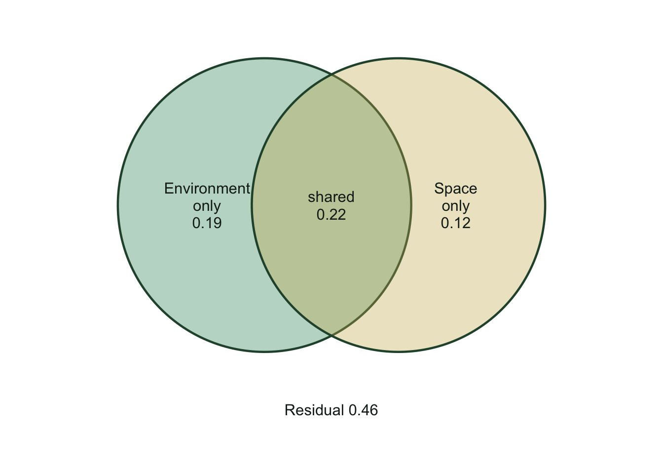
Read the bottom block, the individual fractions. With two tables vegan labels them `[a]` for the part unique to the first table (environment), `[b]` for the part unique to the second (space), `[c]` for the shared fraction, and `[d]` for the residual. Here environment carries the larger unique piece (`[a]`, near 0.19 adjusted R-squared) and space the smaller one (`[b]`, near 0.12), but the shared fraction (`[c]`, near 0.22) is bigger than either of them on its own. Roughly 0.46 stays unexplained.
That shared fraction is the whole point. Notice the partition table near the top: environment on its own (`[a+c]`) explains about 0.42, and space on its own (`[b+c]`) about 0.35. Add those and you get 0.77, far more than the 0.54 the two explain together. The difference is the overlap, counted twice. Variation partitioning shows it once, as `[c]`, and that overlap is exactly the spatially structured environmental signal: moisture varies across space, so the model cannot say whether moisture or position is "responsible" for that slice.
## Why adjusted, and why fractions can go negative
`varpart()` reports adjusted R-squared, not raw. This is not cosmetic. Raw R-squared always rises as you add predictors, so a set with more columns looks more important purely from its size. Peres-Neto, Legendre, Dray and Borcard (2006) showed that the adjusted statistic removes that bias and makes fractions from different-sized tables comparable, which is what lets you put environment (two columns) and space (five columns) on the same axis honestly.
One consequence surprises people: an individual fraction can come out slightly negative. A negative shared fraction is not a bug and not a real "negative variance"; it means the two predictor sets together explain a touch more than the sum of their parts, usually when the sets suppress noise in each other. Report a small negative fraction as effectively zero rather than trying to interpret it.
## Testing the fractions
`varpart()` estimates the fractions but does not test them. For that, drop back to (partial) RDA and permute. The trick is the third argument to `rda()`: it conditions out, that is partials away, a set of variables before testing the rest. Each fraction maps to one model.
```{r}
#| label: tests
# [a+c] environment overall: is environment related to composition at all?
set.seed(1); anova.cca(rda(Yh, env))
# [a] pure environment: environment after removing spatial structure
set.seed(1); anova.cca(rda(Yh, env, space))
# [b] pure space: spatial structure after removing environment
set.seed(1); anova.cca(rda(Yh, space, env))
```
All three are significant at p = 0.001. The pure-environment test (`rda(Yh, env, space)`) is the informative one: even after the trend surface absorbs every smooth spatial gradient, environment still explains a real, independent slice of composition. That is the result you want before claiming an environmental effect, because it rules out the lazy alternative that your "environmental" signal was just spatial autocorrelation in disguise. The pure-space test going significant says the reverse: something spatially structured drives the community that your environmental columns never measured, which is the hidden north-south field by construction.
The shared fraction `[c]` has no such test. It is a difference between two R-squared values, not a model you can fit, so it is descriptive only. The output reminds you of this by marking it `Testable = FALSE`.
## Seeing the split
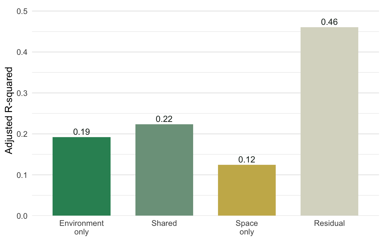
Two pictures carry the result. The Venn shows the fractions in the shape everyone recognises; the bar chart makes their sizes, including the large residual, honest.
```{r}
#| label: venn
#| fig-cap: "Variation partitioning of community composition into pure-environment, pure-space, and shared fractions."
#| fig-width: 7
#| fig-height: 5
fr <- vp$part$indfract
pe <- fr["[a] = X1|X2", "Adj.R.squared"]   # pure environment
ps <- fr["[b] = X2|X1", "Adj.R.squared"]   # pure space
sh <- fr["[c]",          "Adj.R.squared"]  # shared
rs <- fr["[d] = Residuals", "Adj.R.squared"]

circ <- function(cx, cy, r, k = 240) {
  t <- seq(0, 2 * pi, length.out = k)
  data.frame(x = cx + r * cos(t), y = cy + r * sin(t))
}
c1 <- circ(-0.42, 0, 0.92); c1$set <- "Environment"
c2 <- circ( 0.42, 0, 0.92); c2$set <- "Space"
labs <- data.frame(
  x = c(-0.78, 0, 0.78, 0), y = c(0, 0, 0, -1.28),
  lab = c(sprintf("Environment\nonly\n%.2f", pe),
          sprintf("shared\n%.2f", sh),
          sprintf("Space\nonly\n%.2f", ps),
          sprintf("Residual %.2f", rs)))

ggplot() +
  geom_polygon(data = rbind(c1, c2), aes(x, y, group = set, fill = set),
               alpha = 0.35, colour = "#275139", linewidth = 0.8) +
  geom_text(data = labs, aes(x, y, label = lab), size = 4.1,
            colour = "#16241d", lineheight = 0.95) +
  scale_fill_manual(values = c(Environment = "#2f8f63", Space = "#c9b458"),
                    guide = "none") +
  coord_equal(xlim = c(-1.7, 1.7), ylim = c(-1.55, 1.15)) +
  theme_void(base_size = 13)
```
```{r}
#| label: bars
#| fig-cap: "The same four fractions as bars. Most of the variation is unexplained, which is normal for field community data."
#| fig-width: 7
#| fig-height: 4.4
bars <- data.frame(
  fraction = factor(c("Environment\nonly", "Shared", "Space\nonly", "Residual"),
                    levels = c("Environment\nonly", "Shared", "Space\nonly", "Residual")),
  value = c(pe, sh, ps, rs))

ggplot(bars, aes(fraction, value, fill = fraction)) +
  geom_col(width = 0.7) +
  geom_text(aes(label = sprintf("%.2f", value)), vjust = -0.4, size = 4,
            colour = "#16241d") +
  scale_fill_manual(values = c("#2f8f63", "#7ca08a", "#c9b458", "#dad9ca"),
                    guide = "none") +
  scale_y_continuous(expand = expansion(mult = c(0, 0.12))) +
  labs(x = NULL, y = "Adjusted R-squared") +
  theme_minimal(base_size = 13) +
  theme(panel.grid.major.x = element_blank())
```
## What to take away
Variation partitioning answers a question a single R-squared cannot: of the structure in your community, how much belongs uniquely to environment, how much to space, and how much is the spatially organised environment that neither can claim alone. The honest reading of this example is that environment and space each contribute a significant unique fraction, but the largest identified piece is shared, and most of the variation is unexplained, which is the normal state of affairs for field data and worth stating plainly rather than hiding.
Three cautions travel with the method. The shared fraction is descriptive, not a tested effect, so do not write it up as if it were. A trend surface only sees broad gradients; reach for `pcnm()` or dbMEM when spatial structure operates at several scales. And adjusted R-squared is what makes fractions comparable across tables of different sizes, so never partition on raw R-squared.
## References
Borcard, D., Legendre, P. & Drapeau, P. (1992). Partialling out the spatial component of ecological variation. *Ecology*, 73(3), 1045-1055. https://doi.org/10.2307/1940179
Legendre, P. & Gallagher, E.D. (2001). Ecologically meaningful transformations for ordination of species data. *Oecologia*, 129(2), 271-280. https://doi.org/10.1007/s004420100716
Peres-Neto, P.R., Legendre, P., Dray, S. & Borcard, D. (2006). Variation partitioning of species data matrices: estimation and comparison of fractions. *Ecology*, 87(10), 2614-2625. https://doi.org/10.1890/0012-9658(2006)87[2614:VPOSDM]2.0.CO;2