---
title: "Raster data in R with terra: from a DEM to values at your sampling points"
description: "What a raster actually is, how to read its structure, map algebra and slope from an elevation model, what changes when you coarsen the grain, and how to pull raster values out at species points."
date: "2026-06-22 11:00"
categories: [Spatial, Raster data]
image: thumbnail.png
image-alt: "An elevation raster shaded from pale to green, with red species occurrence points scattered over the higher ground."
---
A raster is a grid. Every cell holds one number, the cells are all the same size, and the grid is pinned to the map by an extent and a coordinate reference system. Elevation, temperature, canopy cover, distance to water: anything that varies continuously across space fits this shape. The `terra` package is the current tool for rasters in R, and this post walks the path most ecological work follows: build or read a layer, look at its structure, do arithmetic on it, derive terrain, change its grain, and finally read values off it at the places you sampled.
## Building a raster and reading its structure
A real project starts with `rast("dem.tif")` to read a file. Here we build an elevation model from scratch so the whole post is reproducible. The grid is 100 metre cells over a ten by ten kilometre block, in UTM zone 34N.
```{r}
#| label: build
#| message: false
#| warning: false
library(terra)
library(ggplot2)

set.seed(61)

r <- rast(xmin = 400000, xmax = 410000,
          ymin = 5050000, ymax = 5060000,
          resolution = 100, crs = "EPSG:32634")

# fill the cells with a smooth elevation surface: a regional tilt
# up toward the north, a hill near the middle, and a little noise
xy <- xyFromCell(r, 1:ncell(r))
xs <- (xy[, 1] - 400000) / 10000
ys <- (xy[, 2] - 5050000) / 10000
hill <- exp(-(((xs - 0.45)^2 + (ys - 0.55)^2) / (2 * 0.05)))
values(r) <- 300 + 700 * ys + 250 * xs + 400 * hill + rnorm(ncell(r), 0, 8)
names(r) <- "elevation"
r
```
The printout is the whole identity card of the layer. It is 100 rows by 100 columns, so 10,000 cells, each 100 metres on a side. The extent gives the map coordinates of the outer edges, the coordinate reference system is recorded, and because the values are in memory it shows the range, roughly 300 to 1250 metres here. The accessor functions pull these out one at a time when you need them in code.
```{r}
#| label: accessors
res(r)
ext(r)
global(r, "mean")
```
So the cells are 100 metres, the block sits where the extent says, and the mean elevation is about 890 metres. Keep `global` in mind: it is how you get summary statistics over a whole layer, and it takes `na.rm` like the base functions.
## Map algebra
Arithmetic on a raster works cell by cell. Write the layer into an ordinary expression and `terra` applies it to every cell, returning a new raster on the same grid. A common move is turning elevation into a rough temperature surface with a lapse rate, six degrees cooler for every 1000 metres climbed, off an 18 degree base near sea level.
```{r}
#| label: algebra
tempC <- 18 - 6.0 * (r / 1000)
names(tempC) <- "tempC"
global(tempC, c("min", "max", "mean"))
```
The result is a temperature layer running from about 10.5 degrees on the high ground to a little over 16 degrees in the low corner, averaging about 12.6 degrees. Nothing about the grid changed: same cells, same extent, same reference system, only the values are new. Two layers on the same grid can be combined the same way, which is how you build indices and masks.
## Slope from the elevation model
Some variables are not measured but derived from the shape of the surface. Slope and aspect come straight off a digital elevation model with `terrain`. Because this grid is in metres, the cell spacing is a real distance and slope comes back in sensible degrees.
```{r}
#| label: terrain
slope <- terrain(r, v = "slope", unit = "degrees")
global(slope, c("min", "max", "mean"), na.rm = TRUE)
```
The terrain here is gentle, running from nearly flat to about 15 degrees on the flank of the hill, with a mean near 6 degrees. `terrain` can return aspect, roughness, and other surface descriptors from the same call by changing `v`. One detail worth knowing: on a longitude and latitude grid the cell spacing is not constant, and `terrain` accounts for that internally, but slope is cleaner to reason about on a projected grid like this one.
## Grain: coarsening the raster
The cell size is the grain of your data, and it sets the finest pattern you can see. Coarsening the grain with `aggregate` groups blocks of cells and summarises each block with a function you choose.
```{r}
#| label: aggregate
r500 <- aggregate(r, fact = 5, fun = "mean")
c(res = res(r500)[1], cells = ncell(r500))
global(r500, "mean")
```
Five by five blocks of 100 metre cells give 500 metre cells, so the grid drops from 10,000 cells to 400. The mean elevation barely moves, because averaging blocks and then averaging the blocks returns about the same overall mean. What you lose is the fine detail: the hill is still there at 500 metres, but a narrow gully would be smeared out. Picking a grain is a real modelling decision, not a formatting step, since it fixes the scale of pattern the analysis can detect.
## The payoff: values at sampling points
The reason to hold environmental rasters is usually to attach their values to biological records. You have species occurrences as coordinates, and you want the elevation, temperature, and slope at each one so you can model the niche (Elith & Leathwick 2009). `extract` does exactly that: hand it the layers and a set of points, and it returns one row per point with a column per layer.
```{r}
#| label: extract
#| message: false
#| warning: false
# 80 occurrences of a cool-adapted species, more likely on high ground
p_occ <- plogis((values(r)[, 1] - 750) / 120)
occ_cells <- sample(ncell(r), 80, prob = p_occ)
pts <- vect(xyFromCell(r, occ_cells), type = "points", crs = crs(r))

env <- extract(c(r, tempC, slope), pts)
head(round(env, 2))
```
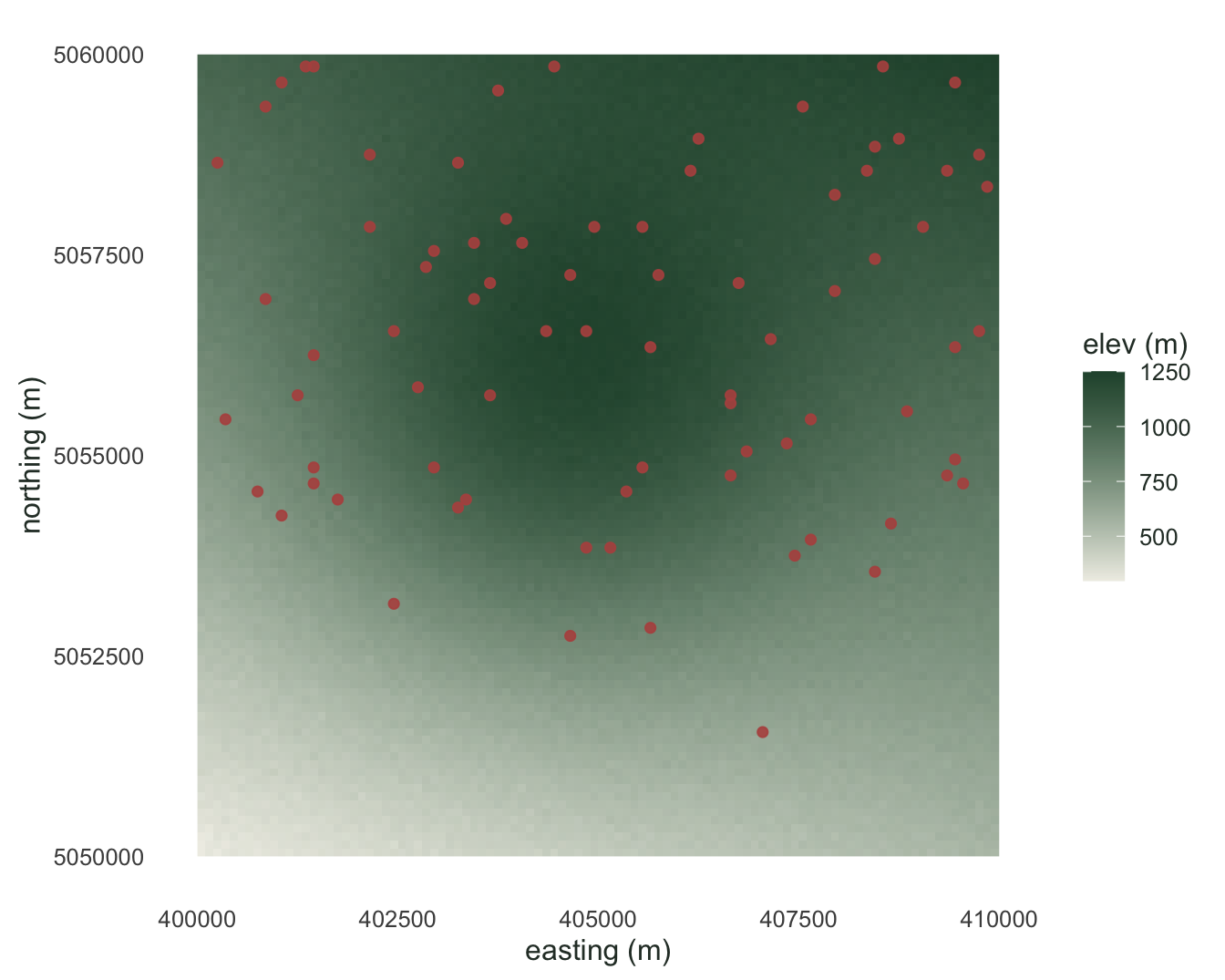
Each point now carries its environmental context, ready for a regression or a distribution model. Because this species was placed to favour high ground, its occurrences should sit above the landscape as a whole, and they do.
```{r}
#| label: compare
c(occ_mean_elev = round(mean(env$elevation), 1),
  land_mean_elev = round(global(r, "mean")[1, 1], 1),
  pct_above_land_mean = round(100 * mean(env$elevation > global(r, "mean")[1, 1])))
```
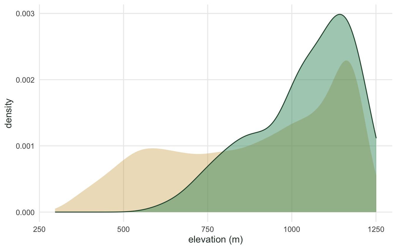
The occurrences average about 1040 metres against roughly 890 for the landscape, and nearly four in five of them fall above the landscape mean. That gap between where a species is and what the whole area offers is the raw material of a species distribution model, and extracting raster values at points is how you put it in a table.
```{r}
#| label: fig-dem
#| message: false
#| warning: false
#| fig-cap: "The elevation raster with the 80 occurrence points in red. Higher ground is darker, and the points lean toward it."
#| fig-alt: "Shaded elevation grid going from pale low ground to dark green high ground, overlaid with scattered red points concentrated on the higher areas."
#| fig-width: 7
#| fig-height: 5.6
df <- as.data.frame(r, xy = TRUE)
ptsdf <- as.data.frame(xyFromCell(r, occ_cells))
names(ptsdf) <- c("x", "y")

ggplot() +
  geom_raster(data = df, aes(x, y, fill = elevation)) +
  geom_point(data = ptsdf, aes(x, y), colour = "#b5534e",
             size = 1.6, alpha = 0.9) +
  scale_fill_gradient(low = "#efeee6", high = "#275139", name = "elev (m)") +
  coord_equal() +
  labs(x = "easting (m)", y = "northing (m)") +
  theme_minimal(base_size = 12) +
  theme(panel.grid = element_blank(),
        text = element_text(colour = "#2c3a31"))
```
```{r}
#| label: fig-extract
#| message: false
#| warning: false
#| fig-cap: "Elevation across the whole landscape (gold) against elevation at the occurrence points (green). The species occupies the upper part of the gradient."
#| fig-alt: "Two overlaid density curves: a broad gold curve over the full elevation range and a green curve shifted toward the high end."
#| fig-width: 7
#| fig-height: 4.4
ggplot() +
  geom_density(data = df, aes(elevation, after_stat(density)),
               fill = "#cda23f", colour = NA, alpha = 0.35) +
  geom_density(data = data.frame(elevation = env$elevation),
               aes(elevation, after_stat(density)),
               fill = "#2f8f63", colour = "#275139", alpha = 0.45) +
  labs(x = "elevation (m)", y = "density") +
  theme_minimal(base_size = 12) +
  theme(panel.grid.minor = element_blank(),
        text = element_text(colour = "#2c3a31"))
```
That is the spine of raster work in `terra`: read a layer and check its structure, compute new layers with map algebra, derive terrain from a surface, choose a grain on purpose, and extract values at the points where the biology was recorded. The vector side of the same workflow, counting records per cell and mapping richness, is in the [species richness mapping](../richness-mapping-sf/) post, and the extracted table here feeds straight into the kind of count model covered in the [GLM post](../glm-count-data-abundance/).
## References
Elith, J., & Leathwick, J. R. (2009). Species distribution models: ecological explanation and prediction across space and time. *Annual Review of Ecology, Evolution, and Systematics*, 40, 677-697. https://doi.org/10.1146/annurev.ecolsys.110308.120159
Hijmans, R. J. (2023). *terra: Spatial Data Analysis*. R package version 1.7-65. https://CRAN.R-project.org/package=terra