Phylogenetic diversity in R: PD, MPD, MNTD

Measure the phylogenetic structure of ecological communities in R with picante: Faith’s PD, mean pairwise distance (MPD) and mean nearest taxon distance (MNTD), standardized effect sizes (NRI and NTI), and why clustering is easier to detect than overdispersion and why the null model decides the answer.

Species richness counts how many species share a site and treats them as interchangeable. Two communities of eight species look identical to it, even if one holds eight close relatives from a single genus and the other holds eight species drawn from across the tree of life. Phylogenetic diversity puts the tree back in. It asks not how many species are present but how much evolutionary history they span, and whether the species that coexist are more closely related, or less, than a random draw from the species pool would be.

This post measures phylogenetic structure with picante (Kembel et al. 2010). It uses three metrics that capture different depths of the tree, standardizes them against a null model to separate signal from richness, and works through two complications that decide what the numbers mean: clustering is easier to detect than overdispersion, and the verdict can flip when you change the null model. That second point is the same lesson as co-occurrence null models, in a phylogenetic key.

A tree and three communities

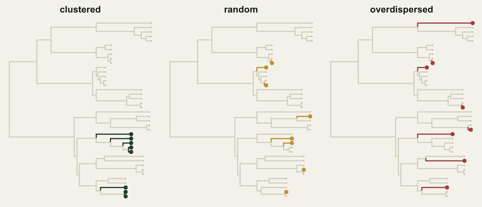
The data are synthetic. The phylogeny has eight genera of five species each, so it has clear clade structure: tips within a genus are close, tips in different genera are distant. The three communities all hold eight species, so richness is held constant and any difference between them is phylogenetic. The clustered community takes its eight species from two neighbouring genera. The overdispersed one takes one species from each of eight genera, spreading across the whole tree. The random one takes eight species at random.

library(ape)
library(picante)
library(ggplot2)
library(dplyr)

build_tree <- function(){
  set.seed(101); genera <- 8; per <- 5
  bb <- rcoal(genera); bb$tip.label <- paste0("G", seq_len(genera))
  full <- bb
  for (g in seq_len(genera)){
    sub <- rcoal(per); sub$tip.label <- paste0("G", g, "_s", seq_len(per))
    sub$edge.length <- sub$edge.length * 0.30
    full <- bind.tree(full, sub, where = which(full$tip.label == paste0("G", g)))
  }
  full <- multi2di(full); full$edge.length[full$edge.length <= 0] <- 1e-6
  full
}
tree <- build_tree()
sp <- tree$tip.label
cophen <- cophenetic(tree)   # patristic distances between all tip pairs

spez <- function(set) as.integer(sp %in% set)
clustered     <- c(paste0("G1_s", 1:5), paste0("G2_s", 1:3))   # two close genera
overdispersed <- paste0("G", 1:8, "_s1")                       # one per genus
set.seed(7); randsp <- sample(sp, 8)                           # random eight
comm <- rbind(clustered = spez(clustered),
              random = spez(randsp),
              overdispersed = spez(overdispersed))
colnames(comm) <- sp

The tree is not ultrametric, which is fine here: the metrics below read pairwise distances off the branches, and do not assume equal root-to-tip lengths. The figure shows the same tree three times, with each community’s eight species marked. The clustered set bunches into two adjacent clades, the overdispersed set spreads one tip per clade down the whole tree, and the random set falls somewhere between.

ink <- "#16241d"; forest_col <- "#275139"; gold <- "#cda23f"; red <- "#b5534e"
fade <- "#c4c8c0"; line_col <- "#dad9ca"; paper <- "#f5f4ee"
tr <- ladderize(tree)
panels <- list(
  list(name = "clustered",     set = clustered,     col = forest_col),
  list(name = "random",        set = randsp,        col = gold),
  list(name = "overdispersed", set = overdispersed, col = red))
par(mfrow = c(1, 3), mar = c(0.5, 0.5, 2.2, 0.5), bg = paper, xpd = NA)
for (m in panels){
  hit <- tr$tip.label %in% m$set
  ec <- rep(line_col, nrow(tr$edge))
  ec[match(which(hit), tr$edge[, 2])] <- m$col
  plot.phylo(tr, show.tip.label = FALSE, edge.color = ec, edge.width = 2.0)
  tiplabels(pch = 16, col = ifelse(hit, m$col, fade),
            cex = ifelse(hit, 1.5, 0.5), tip = seq_len(Ntip(tr)))
  title(main = m$name, col.main = ink, font.main = 2, cex.main = 1.5, line = 0.5)
}

Figure 1: The phylogeny with each community’s eight species marked. Clustering concentrates the sampled tips in two neighbouring clades; overdispersion spreads them evenly across the tree; the random draw sits between the two.

Three metrics for three depths

picante gives three standard measures. Faith’s PD is the total branch length spanned by a community, the sum of all branches needed to connect its species back to the root (Faith 1992). Mean pairwise distance (MPD) averages the patristic distance over every pair of species, which weights the deep, basal splits. Mean nearest taxon distance (MNTD) averages, for each species, the distance to its single closest relative in the community, which weights the shallow, terminal splits. The first two grow with how much history is present; the third tracks how tightly packed the tips are.

pdv   <- pd(comm, tree, include.root = TRUE)
mpdv  <- mpd(comm, cophen, abundance.weighted = FALSE)
mntdv <- mntd(comm, cophen, abundance.weighted = FALSE)
metrics <- data.frame(community = rownames(comm), richness = pdv$SR,
                      PD = round(pdv$PD, 2), MPD = round(mpdv, 2), MNTD = round(mntdv, 2))
metrics

      community richness   PD  MPD MNTD
1     clustered        8 3.02 0.86 0.28
2        random        8 5.85 1.97 0.86
3 overdispersed        8 7.22 2.30 1.25

All three communities have richness eight, yet Faith’s PD runs 3.0, 5.9 and 7.2 from clustered to overdispersed. The clustered community packs eight species into a sliver of the tree and spans the least history; the overdispersed one reaches across the tree and spans the most. MPD and MNTD tell the same ordering at different depths: clustered species are close on average (MPD 0.86) and have very near nearest-relatives (MNTD 0.28), while the overdispersed species are distant on both counts.

The trouble with reading these raw numbers is that PD positively correlates with richness, so on real data, where richness varies between sites, you cannot tell whether a high PD means a community spans more history or simply holds more species. The fix is to standardize: compare the observed value against the distribution you would get by assembling random communities of the same richness from the species pool.

Standardizing: effect sizes and the null distribution

ses.mpd and ses.mntd do exactly this. They shuffle species across the tips of the tree many times, recompute the metric for a community of the same richness on each shuffle, and report the standardized effect size: observed minus the null mean, over the null standard deviation. By convention these are reported with the sign flipped and named the net relatedness index (NRI, from MPD) and the nearest taxon index (NTI, from MNTD), so that a positive index means clustering (Webb et al. 2002). To avoid sign confusion this post keeps the raw effect size: negative means clustered, positive means overdispersed.

set.seed(42); smpd  <- ses.mpd(comm,  cophen, null.model = "taxa.labels", runs = 999)
set.seed(42); smntd <- ses.mntd(comm, cophen, null.model = "taxa.labels", runs = 999)
data.frame(community = rownames(comm),
           mpd.z = round(smpd$mpd.obs.z, 2),   mpd.p = smpd$mpd.obs.p,
           mntd.z = round(smntd$mntd.obs.z, 2), mntd.p = smntd$mntd.obs.p)

      community mpd.z mpd.p mntd.z mntd.p
1     clustered -7.10 0.001  -2.86  0.004
2        random -0.85 0.166  -0.13  0.459
3 overdispersed  1.03 0.874   1.70  0.964

The clustered community is strongly and significantly clustered on both metrics: MPD effect size -7.1 (p = 0.001) and MNTD effect size -2.9 (p = 0.004). The random community sits inside the null on both, as it should. The overdispersed community is positive on both metrics, MPD +1.0 and MNTD +1.7, the right direction, but neither clears the conventional two-sided threshold of about two standard deviations. A community built to be overdispersed is not flagged as significantly overdispersed.

The null distribution shows why. Because all three communities have richness eight, they share one null distribution: the spread of MPD over random eight-species draws from this tree. Plotting it with the three observed values marked makes the asymmetry visible.

faint <- "#5d6b61"
te <- theme_minimal(base_size = 12) + theme(
  panel.grid.minor = element_blank(),
  panel.grid.major = element_line(color = line_col, linewidth = 0.3),
  plot.background = element_rect(fill = paper, color = NA),
  panel.background = element_rect(fill = paper, color = NA),
  axis.title = element_text(color = "#46604a"),
  legend.position = "top", legend.title = element_blank())

set.seed(42)
draws <- replicate(999, mpd(comm, taxaShuffle(cophen)))   # one row per community, identical in distribution
nulls <- data.frame(MPD = as.vector(draws))
obs <- data.frame(
  community = factor(rownames(comm), levels = c("clustered", "random", "overdispersed")),
  MPD = as.numeric(mpdv), z = round(smpd$mpd.obs.z, 1))
cols <- c(clustered = forest_col, random = gold, overdispersed = red)
obs$lab <- sprintf("%s\nSES %.1f", obs$community, obs$z)

ggplot(nulls, aes(MPD)) +
  geom_histogram(bins = 40, fill = line_col, color = paper, linewidth = 0.15) +
  geom_vline(data = obs, aes(xintercept = MPD, color = community), linewidth = 1.0) +
  geom_text(data = obs, aes(x = MPD, y = Inf, label = lab, color = community),
            angle = 90, hjust = 1.05, vjust = -0.35, size = 3.0, lineheight = 0.9,
            show.legend = FALSE) +
  scale_color_manual(values = cols) +
  labs(x = "mean pairwise distance (MPD) under taxa.labels null", y = "simulations") +
  coord_cartesian(xlim = c(0.4, 2.7)) + te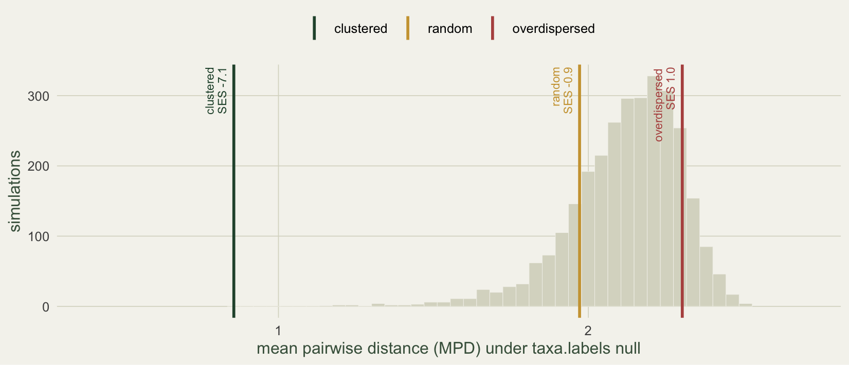

Figure 2: Null distribution of MPD for random eight-species communities, with the three observed values marked. The distribution is left-skewed, so the clustered community falls far into the long left tail and is easily significant, while the overdispersed community is pressed against the compressed right edge and is not.

The null distribution is left-skewed. Random draws of eight species from this tree almost always span several genera, so their MPD piles up near the high end, and the distribution trails off to the left toward the rare draws that happen to be closely related. A clustered community lands in that long left tail, far from the bulk, and is easy to flag. An overdispersed community can only push to the right, against the compressed upper edge where there is little room to be unusual. This is a documented asymmetry: phylogenetic clustering is generally easier to detect than overdispersion, and detection power for overdispersion is low (Kembel 2009).

Basal versus terminal, and which null

The two effect sizes are not redundant. MPD reads the deep structure of the tree, MNTD the shallow. A community can be clustered at the tips while ordinary at the base, or the reverse. The figure puts both side by side, with the band marking the non-significant zone.

bandfill <- "#e8e7dc"
ses_df <- bind_rows(
  data.frame(community = rownames(comm), metric = "MPD (basal)", z = smpd$mpd.obs.z),
  data.frame(community = rownames(comm), metric = "MNTD (tip)",  z = smntd$mntd.obs.z))
ses_df$community <- factor(ses_df$community, levels = c("overdispersed", "random", "clustered"))
ses_df$metric <- factor(ses_df$metric, levels = c("MPD (basal)", "MNTD (tip)"))
ses_df$sig <- ifelse(abs(ses_df$z) > 1.96, "p < 0.05", "n.s.")

ggplot(ses_df, aes(z, community)) +
  annotate("rect", xmin = -1.96, xmax = 1.96, ymin = -Inf, ymax = Inf,
           fill = bandfill, alpha = 0.7) +
  geom_vline(xintercept = 0, color = faint, linewidth = 0.4) +
  geom_segment(aes(x = 0, xend = z, yend = community), color = line_col, linewidth = 1.1) +
  geom_point(aes(color = sig), size = 4) +
  scale_color_manual(values = c(`p < 0.05` = forest_col, `n.s.` = faint)) +
  scale_x_continuous(limits = c(-8.2, 3.2), breaks = seq(-8, 2, 2)) +
  facet_wrap(~metric) +
  labs(x = "standardized effect size (negative = clustered, positive = overdispersed)",
       y = NULL) +
  te + theme(panel.grid.major.y = element_blank())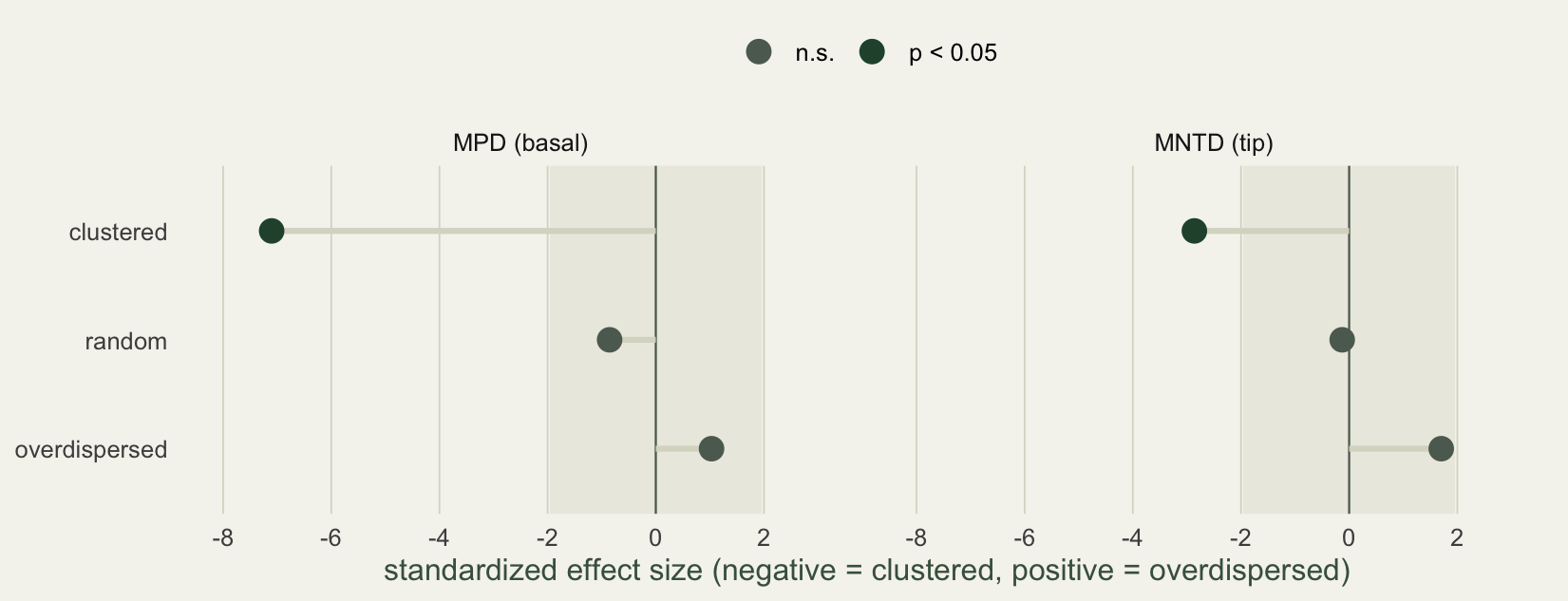

Figure 3: Standardized effect sizes for MPD (deep, basal structure) and MNTD (shallow, terminal structure). The clustered community is significant at both depths; the directional gradient from overdispersed to clustered is visible in both panels; the shaded band marks effect sizes within about two standard deviations of the null.

For the clustered community the basal signal (effect size -7.1) is much stronger than the terminal one (-2.9). The eight species come from two whole genera, so they are deeply clustered across the tree, while within those genera the nearest-relative distances are less extreme. Reading both metrics tells you not just that a community is clustered but at what depth, which is information a single number hides.

The choice of null model matters as much as the choice of metric, and here the post meets the same fork as co-occurrence analysis. The taxa.labels null used above draws random species from the pool with every species equally likely. The independentswap null instead shuffles the community matrix while preserving both site richness and each species’ occurrence frequency, the phylogenetic analogue of the fixed-fixed model for co-occurrence.

set.seed(42); is_mpd <- ses.mpd(comm, cophen, null.model = "independentswap", runs = 999)
data.frame(community = rownames(comm),
           taxa.labels = round(smpd$mpd.obs.z, 2),
           independentswap = round(is_mpd$mpd.obs.z, 2))

      community taxa.labels independentswap
1     clustered       -7.10           -4.25
2        random       -0.85            0.61
3 overdispersed        1.03            2.02

The clustering signal holds under both nulls. The overdispersion result does not: under taxa.labels the overdispersed community sits at effect size +1.0, inside the null, but under independentswap it moves to +2.0, just across the threshold. Preserving the occurrence frequencies tightens the null and makes the same observed value look more extreme. With only three communities the independentswap null has little room to rearrange, so treat this particular crossing as an illustration of the principle rather than a firm result: the null model is part of the hypothesis, and a borderline pattern can land on either side of significance depending on which one you choose.

How far to read these patterns

The standard reading maps clustering onto habitat filtering, where an environment admits only species with the right, and therefore shared and conserved, traits, and overdispersion onto competition, where close relatives exclude one another. Both readings assume the ecologically relevant traits are themselves phylogenetically conserved, so that relatedness stands in for ecological similarity (Webb et al. 2002). When that assumption fails the metrics still compute but the inference does not follow, and the link from overdispersion to competition in particular has thin empirical support. A significant effect size is a statement about phylogenetic pattern, not a measured process.

A few practical notes. Set a seed before each ses.* call, since the effect size and its p-value come from a finite number of shuffles. Report the effect size alongside the p-value: with 999 runs the smallest attainable p-value is about 0.001, and a near-threshold result like the overdispersed community here is better described by its effect size than forced into a significant-or-not verdict. The metrics accept abundance weighting through abundance.weighted = TRUE, which shifts MPD and MNTD toward the dominant species much as abundance weighting changes functional dispersion. And the tree need not be ultrametric for distance-based metrics, but if you compute Faith’s PD the position of the root matters, so decide deliberately whether include.root belongs in your question.

References

Faith DP (1992). Conservation evaluation and phylogenetic diversity. Biological Conservation 61(1):1-10. doi:10.1016/0006-3207(92)91201-3

Webb CO, Ackerly DD, McPeek MA, Donoghue MJ (2002). Phylogenies and community ecology. Annual Review of Ecology and Systematics 33:475-505. doi:10.1146/annurev.ecolsys.33.010802.150448

Kembel SW (2009). Disentangling niche and neutral influences on community assembly: assessing the performance of community phylogenetic structure tests. Ecology Letters 12(9):949-960. doi:10.1111/j.1461-0248.2009.01354.x

Kembel SW, Cowan PD, Helmus MR, et al. (2010). Picante: R tools for integrating phylogenies and ecology. Bioinformatics 26(11):1463-1464. doi:10.1093/bioinformatics/btq166