Mantel tests in R: correlating distance matrices, and when not to

Simple and partial Mantel tests with vegan, what they actually test, and why a spatially structured environment can make geography look important when it is not.

A Mantel test asks whether two distance matrices covary. In community ecology the usual version is: do sites that differ a lot in their environment also differ a lot in species composition? A partial Mantel adds a third matrix, so you can ask the same question while holding geographic distance constant. The mechanics are a couple of lines in vegan. The interpretation is where most of the trouble lives, so the last section is about what the test really answers and where it tends to mislead.

A landscape where environment and space are tangled

The example uses 50 sites on a unit square. Soil moisture rises from west to east, so moisture carries a spatial pattern of its own. Eighteen species have Gaussian responses to moisture, and a second driver that we never measure also shapes part of the community. That second driver matters: a single measured gradient never explains everything in real data, and leaving some composition unexplained by moisture keeps the example honest.

library(vegan)
library(ggplot2)

set.seed(33)

n_sites <- 50
x <- runif(n_sites)
y <- runif(n_sites)

# moisture: west-east gradient (spatial), mild north-south, plus noise
moisture <- 60 + 25 * x + 6 * y + rnorm(n_sites, 0, 6)

# a second driver, not spatially structured and not measured.
# some species track it, so moisture explains only part of the pattern.
z <- rnorm(n_sites, 0, 1)

n_sp   <- 18
opt    <- seq(52, 98, length.out = n_sp)   # moisture optima
width  <- 10
peak   <- 18
z_load <- c(rep(0, 9), runif(9, 0.5, 1.1)) # last nine species respond to z

log_lambda <- outer(moisture, opt,
                    function(m, o) log(peak) - ((m - o)^2) / (2 * width^2)) +
  outer(z, z_load)
comm <- matrix(rpois(n_sites * n_sp, exp(log_lambda)), nrow = n_sites)
colnames(comm) <- paste0("sp", seq_len(n_sp))

The moisture gradient is easy to see when you put the sites back on the map.

map_df <- data.frame(x = x, y = y, moisture = moisture)

ggplot(map_df, aes(x, y, fill = moisture)) +
  geom_point(shape = 21, size = 5, colour = "#2c3a31", stroke = 0.5) +
  scale_fill_gradient(low = "#c9b458", high = "#1d5b4e", name = "Soil\nmoisture") +
  coord_equal() +
  labs(x = "Easting (unit square)", y = "Northing (unit square)") +
  theme_minimal(base_size = 13) +
  theme(panel.grid.minor = element_blank(),
        text = element_text(colour = "#2c3a31"))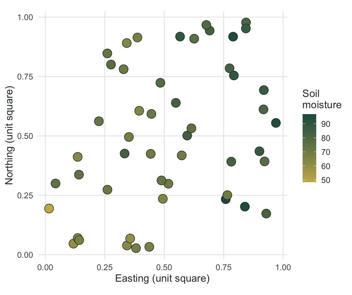

Figure 1: The 50 sites, coloured by soil moisture. Moisture rises from west to east, so it is itself a spatial variable. That is the property that will make geography look important later.

Three distance matrices

A Mantel test never sees the site values directly. It works on distances: one matrix per data source, each holding the pairwise distance between every pair of sites. Here we need three.

comm_d <- vegdist(comm, method = "bray")   # community dissimilarity
env_d  <- dist(scale(moisture))            # environmental distance
geo_d  <- dist(cbind(x, y))                # geographic distance

Community dissimilarity is Bray-Curtis on the abundances. Environmental distance is the absolute difference in scaled moisture. Geographic distance is the straight-line distance on the map. Every Mantel test below is a correlation between two of these three, computed over the lower triangle of the matrices.

The simple Mantel test

Start with the question people usually ask: is community dissimilarity related to environmental distance?

set.seed(33)
mantel(comm_d, env_d, method = "pearson", permutations = 999)

Mantel statistic based on Pearson's product-moment correlation 

Call:
mantel(xdis = comm_d, ydis = env_d, method = "pearson", permutations = 999) 

Mantel statistic r: 0.7579 
      Significance: 0.001 

Upper quantiles of permutations (null model):
  90%   95% 97.5%   99% 
0.085 0.112 0.138 0.162 
Permutation: free
Number of permutations: 999

The correlation comes out around 0.76 with a permutation p of 0.001. Sites that differ in moisture differ in composition, which is what the data were built to show. Now run the same test against geographic distance.

set.seed(33)
mantel(comm_d, geo_d, method = "pearson", permutations = 999)

Mantel statistic based on Pearson's product-moment correlation 

Call:
mantel(xdis = comm_d, ydis = geo_d, method = "pearson", permutations = 999) 

Mantel statistic r: 0.324 
      Significance: 0.001 

Upper quantiles of permutations (null model):
   90%    95%  97.5%    99% 
0.0610 0.0883 0.1074 0.1234 
Permutation: free
Number of permutations: 999

This one is positive too, around 0.32 and again significant. Read on its own, that result invites a story about dispersal limitation or spatial structure in the community. Before accepting it, check whether the environment is itself spatial.

set.seed(33)
mantel(env_d, geo_d, method = "pearson", permutations = 999)

Mantel statistic based on Pearson's product-moment correlation 

Call:
mantel(xdis = env_d, ydis = geo_d, method = "pearson", permutations = 999) 

Mantel statistic r: 0.4036 
      Significance: 0.001 

Upper quantiles of permutations (null model):
   90%    95%  97.5%    99% 
0.0626 0.0802 0.0962 0.1114 
Permutation: free
Number of permutations: 999

Environmental distance and geographic distance correlate at about 0.40. Moisture is patterned in space, so two sites that are far apart tend to differ in moisture, and therefore in composition. The community-geography correlation might be nothing more than the spatial footprint of moisture. The scatterplots make the difference in signal plain.

set.seed(33)
r_env <- mantel(comm_d, env_d, permutations = 999)$statistic
set.seed(33)
r_geo <- mantel(comm_d, geo_d, permutations = 999)$statistic

dd_long <- data.frame(
  comm = rep(as.vector(comm_d), 2),
  dist = c(as.vector(env_d), as.vector(geo_d)),
  type = rep(c(
    sprintf("community vs environment   (Mantel r = %.2f)", r_env),
    sprintf("community vs geography   (Mantel r = %.2f)", r_geo)
  ), each = length(comm_d))
)

ggplot(dd_long, aes(dist, comm)) +
  geom_point(alpha = 0.22, colour = "#275139", size = 1.2) +
  geom_smooth(method = "lm", se = FALSE, colour = "#b5534e", linewidth = 1) +
  facet_wrap(~ type, scales = "free_x") +
  labs(x = "Pairwise distance between sites",
       y = "Community dissimilarity (Bray-Curtis)") +
  theme_minimal(base_size = 12) +
  theme(panel.grid.minor = element_blank(),
        strip.text = element_text(face = "bold", size = 10),
        text = element_text(colour = "#2c3a31"))

`geom_smooth()` using formula = 'y ~ x'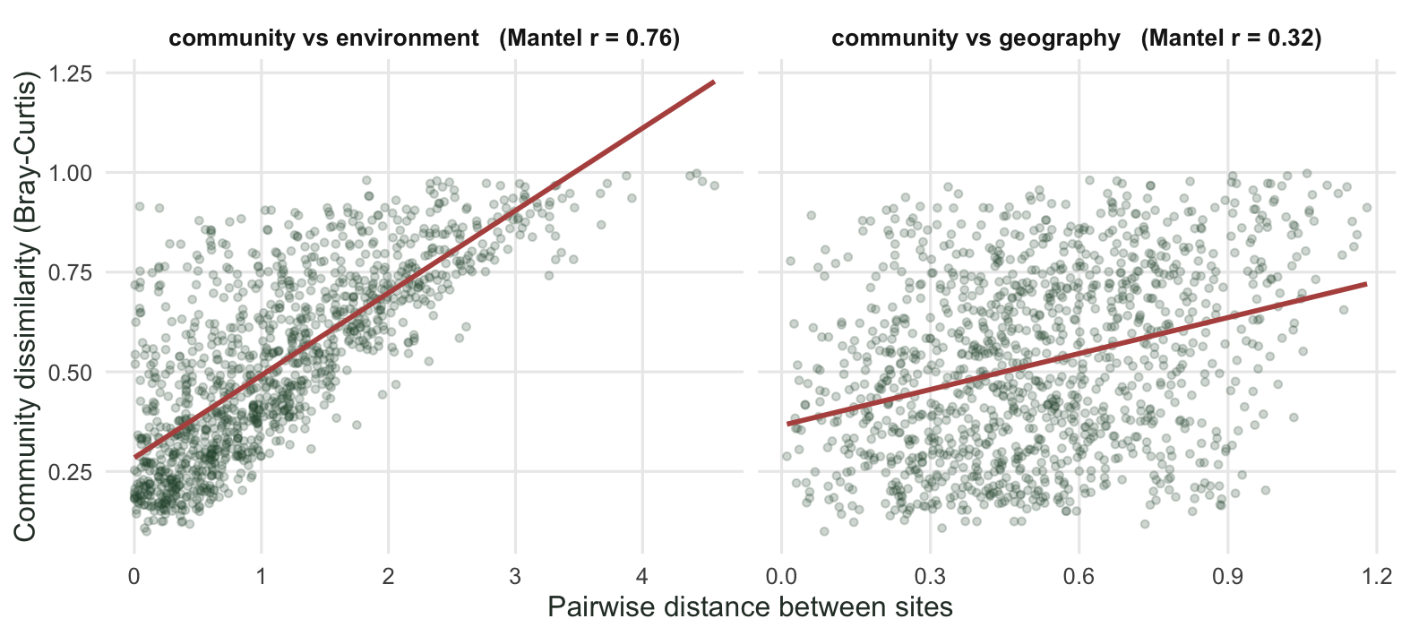

Figure 2: What a Mantel test correlates. Each point is one pair of sites: its distance on the x axis against its community dissimilarity on the y axis. The community-environment relationship (left) is much tighter than the community-geography relationship (right). The red line is the linear fit that the Pearson Mantel statistic summarises.

The partial Mantel test

A partial Mantel correlates two matrices while holding a third constant, in the same spirit as partial correlation on ordinary variables. mantel.partial() takes the three matrices in order: the two being correlated, then the one being controlled for.

set.seed(33)
mantel.partial(comm_d, env_d, geo_d, method = "pearson", permutations = 999)

Partial Mantel statistic based on Pearson's product-moment correlation 

Call:
mantel.partial(xdis = comm_d, ydis = env_d, zdis = geo_d, method = "pearson",      permutations = 999) 

Mantel statistic r: 0.7245 
      Significance: 0.001 

Upper quantiles of permutations (null model):
   90%    95%  97.5%    99% 
0.0862 0.1093 0.1368 0.1592 
Permutation: free
Number of permutations: 999

Controlling for geography, the community-environment correlation barely moves, from about 0.76 down to about 0.73. The moisture signal is not an artefact of space. Now reverse the roles and control for the environment instead.

set.seed(33)
mantel.partial(comm_d, geo_d, env_d, method = "pearson", permutations = 999)

Partial Mantel statistic based on Pearson's product-moment correlation 

Call:
mantel.partial(xdis = comm_d, ydis = geo_d, zdis = env_d, method = "pearson",      permutations = 999) 

Mantel statistic r: 0.03033 
      Significance: 0.27 

Upper quantiles of permutations (null model):
   90%    95%  97.5%    99% 
0.0702 0.0877 0.1019 0.1228 
Permutation: free
Number of permutations: 999

The community-geography correlation collapses to about 0.03 with a p near 0.27, no longer distinguishable from zero. The apparent role of distance was borrowed entirely from moisture. That matches the simulation: nothing connects composition to raw coordinates except through moisture, and once moisture is held constant, position on the map carries almost no information about which species are present.

What the Mantel test actually tests

This is the part to read twice. The result above is clean because the data were built for it, but the same machinery gets used on real data to answer a question it was not designed for, and the literature has been clear about the problem for over a decade.

The null hypothesis of a Mantel test is not the null hypothesis of an ordinary correlation. A Pearson correlation between two variables asks whether the variables themselves are associated. A Mantel test asks whether the distances derived from them are associated. Those are different questions, the test statistics behave differently, and rejecting one null does not imply rejecting the other (Legendre, Fortin & Borcard 2015).

For the specific and very common goal of testing a species-environment relationship while accounting for space, that gap has real consequences. Simulation studies show that when both matrices carry spatial autocorrelation, the simple and partial Mantel tests can have inflated type I error and low power, and the partial test does not fix the bias the way people assume it does (Guillot & Rousset 2013; Legendre, Fortin & Borcard 2015). The recommended alternative is to bring space into the model directly, as spatial eigenfunctions (distance-based Moran eigenvector maps), and then partition the variation with redundancy analysis. The variation partitioning post walks through that workflow, and the dbRDA post covers the constrained ordination it rests on.

So when is a Mantel test the right tool? When distances are genuinely the objects of study rather than a stand-in for variables. Isolation by distance in population genetics fits, because the hypothesis is literally about genetic distance against geographic distance. Comparing two independently measured dissimilarity matrices fits, for example asking whether morphological distance tracks genetic distance. And describing the scale of community turnover fits: a Mantel correlogram, available as mantel.correlog() in vegan, shows how community similarity decays across distance classes, which is more informative than a single coefficient. Reach for the Mantel test when the question is about distances. When the question is about variables and you want to control for space, partition variation instead.

References

Guillot, G., & Rousset, F. (2013). Dismantling the Mantel tests. Methods in Ecology and Evolution, 4(4), 336-344. https://doi.org/10.1111/2041-210x.12018

Legendre, P., Fortin, M.-J., & Borcard, D. (2015). Should the Mantel test be used in spatial analysis? Methods in Ecology and Evolution, 6(11), 1239-1247. https://doi.org/10.1111/2041-210X.12425

Mantel, N. (1967). The detection of disease clustering and a generalized regression approach. Cancer Research, 27(2), 209-220.

Smouse, P. E., Long, J. C., & Sokal, R. R. (1986). Multiple regression and correlation extensions of the Mantel test of matrix correspondence. Systematic Zoology, 35(4), 627-632. https://doi.org/10.2307/2413122