library(indicspecies)
library(dplyr)
library(tidyr)
library(ggplot2)

set.seed(7)
habitats <- rep(c("Forest", "Grassland", "Wetland"), each = 8)   # 24 sites

make_sp <- function(means_by_hab) {
  sapply(habitats, function(h) rpois(1, means_by_hab[[h]]))
}
sp_list <- list(
  For1 = c(Forest=10,Grassland=0, Wetland=0), For2 = c(Forest=9, Grassland=0, Wetland=0),
  For3 = c(Forest=11,Grassland=0, Wetland=0), For4 = c(Forest=8, Grassland=0, Wetland=1),
  Gra1 = c(Forest=0, Grassland=10,Wetland=0), Gra2 = c(Forest=0, Grassland=9, Wetland=0),
  Gra3 = c(Forest=1, Grassland=11,Wetland=0), Gra4 = c(Forest=0, Grassland=8, Wetland=0),
  Wet1 = c(Forest=0, Grassland=0, Wetland=10),Wet2 = c(Forest=0, Grassland=0, Wetland=9),
  Wet3 = c(Forest=0, Grassland=1, Wetland=11),Wet4 = c(Forest=0, Grassland=0, Wetland=8),
  FoGr1= c(Forest=7, Grassland=7, Wetland=0), FoGr2= c(Forest=8, Grassland=6, Wetland=0),
  Gen1 = c(Forest=5, Grassland=5, Wetland=5), Gen2 = c(Forest=6, Grassland=4, Wetland=5),
  Gen3 = c(Forest=4, Grassland=5, Wetland=6),
  Rar1 = c(Forest=0.4,Grassland=0.4,Wetland=0.4), Rar2 = c(Forest=0.3,Grassland=0.5,Wetland=0.3),
  Rar3 = c(Forest=0.5,Grassland=0.3,Wetland=0.4)
)
comm <- as.data.frame(lapply(sp_list, make_sp))
rownames(comm) <- paste0(substr(habitats, 1, 1),
ave(seq_along(habitats), habitats, FUN = seq_along))Indicator species analysis in R: which species characterize your groups
community ecology
indicator species
R
PERMANOVA tells you groups differ. Indicator species analysis tells you which species drive the difference. A walk through multipatt, the IndVal index, and its specificity and fidelity components.
A PERMANOVA or an ordination can tell you that communities in different groups are not the same. That is a useful result, but it is also where most analyses stop, one step short of the question a field ecologist actually wants answered: which species make those groups different? Indicator species analysis fills that gap. It asks, for every species, whether it is a reliable marker of a particular group of sites, and it gives a number and a p-value for the claim.
This post runs indicator species analysis in R with the indicspecies package, focusing on its multipatt function and the IndVal index behind it (Dufrêne and Legendre 1997; De Cáceres and Legendre 2009).
What IndVal measures
The indicator value of a species for a group combines two ideas that ecologists already think in terms of.
Specificity (A) asks: when this species shows up, how often is it in this group rather than elsewhere? A species found only in wetlands has high specificity for wetlands. If most of its abundance sits in one group, A is close to 1.
Fidelity (B) asks: within this group, how many of the sites actually contain the species? A species present in every wetland site has high fidelity, even if it occasionally turns up elsewhere. If it is in all the group’s sites, B is close to 1.
A good indicator needs both. A species can be perfectly faithful to a group (in all its sites) yet useless as a marker if it is also everywhere else (low specificity). The IndVal index multiplies the two, so it is only high when a species is both concentrated in the group and consistently present across it. multipatt with the group-equalized variant reports the statistic as the square root of the product, so the value stays on a 0 to 1 scale.
Beyond single groups: multipatt
Classic indicator analysis tests each species against each group on its own. The multipatt extension (De Cáceres, Legendre and Moretti 2010) adds something useful: it also tests species against combinations of groups. A species might not be a clean marker of forest or of grassland alone, but it might be a strong marker of forest-and-grassland together, separating both from wetland. Real species often behave this way, tracking a broad habitat type rather than one narrow category, and multipatt can name that pattern instead of forcing the species into a single group or discarding it.
A worked example
Here is a synthetic dataset with 24 sites split evenly across three habitats and 20 species built to cover the cases that come up in practice: four specialists for each habitat, two species shared by forest and grassland, three generalists found everywhere, and three rare species that are mostly noise. The data is synthetic and illustrative.
The heatmap makes the design legible. Each specialist block lights up in one habitat, the forest-and-grassland pair lights up in two, the generalists hum along at moderate abundance everywhere, and the rare species are barely there.
hm <- comm %>% mutate(site = rownames(comm), habitat = habitats) %>%
  pivot_longer(-c(site, habitat), names_to = "species", values_to = "abund")
hm$site    <- factor(hm$site, levels = rev(rownames(comm)))
hm$species <- factor(hm$species, levels = colnames(comm))
hm$habitat <- factor(hm$habitat, levels = c("Forest","Grassland","Wetland"))

ggplot(hm, aes(species, site, fill = abund)) +
  geom_tile(color = "white", linewidth = 0.3) +
  facet_grid(habitat ~ ., scales = "free_y", space = "free_y", switch = "y") +
  scale_fill_gradient(low = "#f5f4ee", high = "#275139", name = "abundance") +
  labs(x = NULL, y = NULL) +
  theme_minimal(base_size = 12) +
  theme(panel.grid = element_blank(),
        axis.text.x = element_text(angle = 45, hjust = 1, size = 9),
        strip.placement = "outside", legend.position = "top")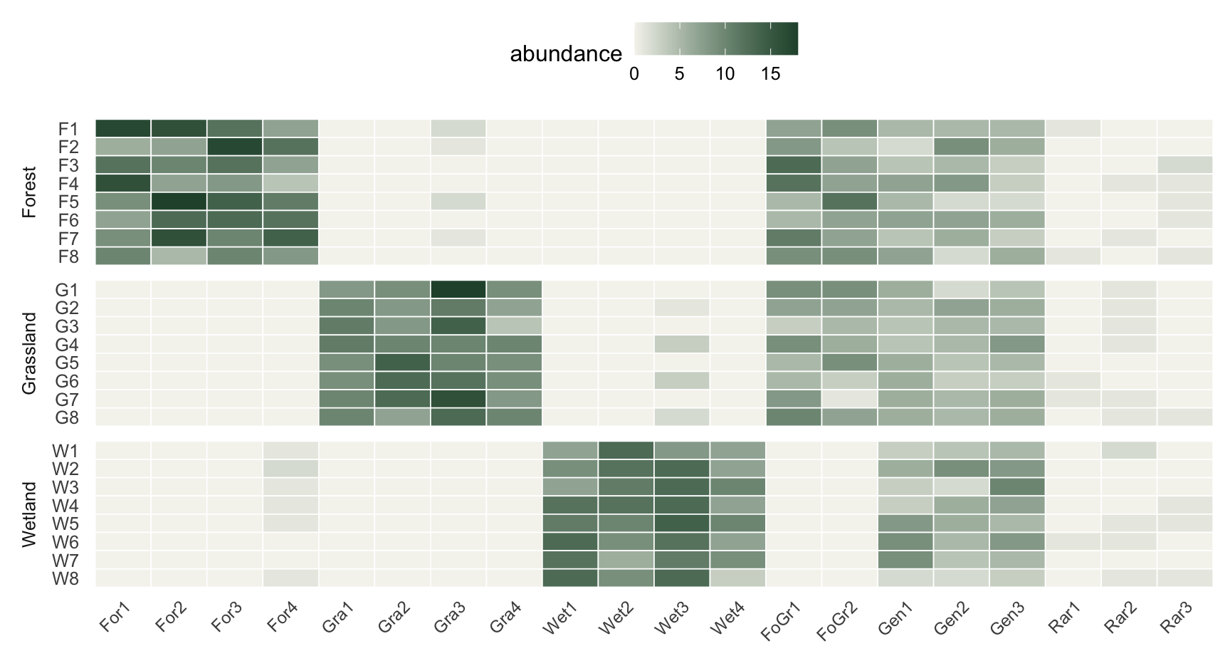
Running multipatt
The call needs three things: the community table, the grouping vector, and a permutation setup. The func = "IndVal.g" argument selects the group-equalized index, which De Cáceres recommends because it does not let unequal group sizes distort the result. The permutation test is what turns each indicator value into a p-value, so set a seed first to make those p-values reproducible.
set.seed(42)   # fixes the permutation p-values
res <- multipatt(comm, habitats, func = "IndVal.g", control = how(nperm = 999))
summary(res)
 Multilevel pattern analysis
 ---------------------------

 Association function: IndVal.g
 Significance level (alpha): 0.05

 Total number of species: 20
 Selected number of species: 14
 Number of species associated to 1 group: 12
 Number of species associated to 2 groups: 2

 List of species associated to each combination:

 Group Forest  #sps.  4
      stat p.value
For1 1.000   0.001 ***
For2 1.000   0.001 ***
For3 1.000   0.001 ***
For4 0.956   0.001 ***

 Group Grassland  #sps.  4
      stat p.value
Gra1 1.000   0.001 ***
Gra2 1.000   0.001 ***
Gra4 1.000   0.001 ***
Gra3 0.972   0.001 ***

 Group Wetland  #sps.  4
      stat p.value
Wet1 1.000   0.001 ***
Wet2 1.000   0.001 ***
Wet4 1.000   0.001 ***
Wet3 0.957   0.001 ***

 Group Forest+Grassland  #sps.  2
      stat p.value
FoGr1    1   0.001 ***
FoGr2    1   0.001 ***
---
Signif. codes:  0 '***' 0.001 '**' 0.01 '*' 0.05 '.' 0.1 ' ' 1
summary() prints the significant indicators grouped by what they indicate: first the species tied to single habitats, then any species tied to a combination. The output here recovers the design cleanly. Twelve specialists land in their own habitats, and the two shared species, FoGr1 and FoGr2, are reported together under the forest-and-grassland combination rather than being split or dropped. Every significant indicator comes in at p = 0.001, the smallest value 999 permutations can produce.
Reading the results
It helps to pull the indicator value apart into the specificity (A) and fidelity (B) components, because that is where the ecology lives. The full res$sign table carries the chosen combination and statistic for every species; res$A and res$B hold the components.
idx <- res$sign$index
lab <- colnames(res$comb)[idx]
A_best <- sapply(seq_along(idx), function(i) res$A[i, idx[i]])
B_best <- sapply(seq_along(idx), function(i) res$B[i, idx[i]])
ind <- data.frame(species = rownames(res$sign), cluster = lab,
                  A = A_best, B = B_best, stat = res$sign$stat, p = res$sign$p.value)
ind <- ind[!is.na(ind$p) & ind$p <= 0.05, ]

clust_cols <- c("Forest"="#275139","Grassland"="#7d8a3c",
                "Wetland"="#3a7ca5","Forest+Grassland"="#c98a2e")
ind$cluster <- factor(ind$cluster, levels = names(clust_cols))
ind <- ind[order(ind$cluster, ind$stat), ]
ind$species <- factor(ind$species, levels = ind$species)

ggplot(ind, aes(stat, species, color = cluster)) +
  geom_segment(aes(x = 0, xend = stat, yend = species), linewidth = 0.6) +
  geom_point(size = 3) +
  scale_color_manual(values = clust_cols, name = "indicates") +
  scale_x_continuous(limits = c(0, 1.05), breaks = seq(0, 1, 0.25)) +
  labs(x = "IndVal stat", y = NULL) +
  theme_minimal(base_size = 12) + theme(legend.position = "right")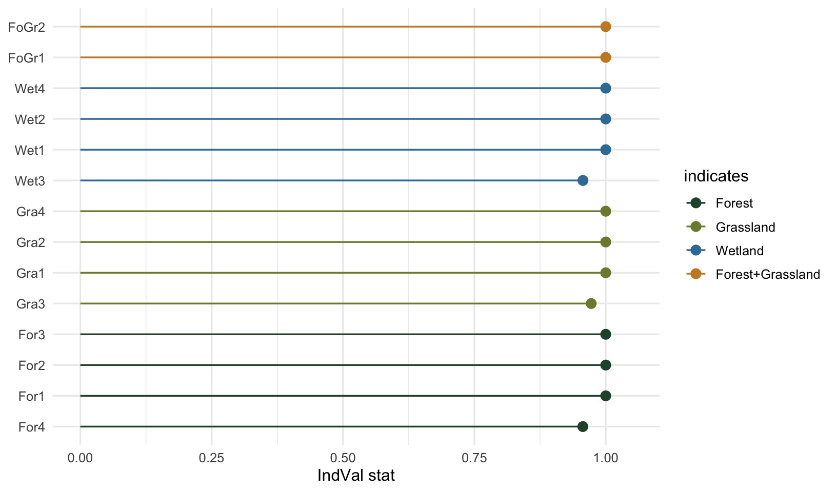
Most indicators here sit at or near the maximum because the synthetic specialists are clean. The three that fall slightly short, For4, Gra3 and Wet3, are the ones I let appear once in a neighbouring habitat, which trims their specificity (A) below 1 while their fidelity (B) stays at 1. That is the component view earning its keep: it tells you a marginally lower indicator value came from a small loss of specificity, not from patchy presence within the group.
What about the generalists and the noise
The interesting part of this output is what is not in the significant list. The three generalists never appear, and neither do the rare species. Looking at their rows explains why.
res$sign[c("Gen1","Gen3","Rar1","Rar2"), ] s.Forest s.Grassland s.Wetland index stat p.value
Gen1 1 1 1 7 1.0000000 NA
Gen3 1 1 1 7 1.0000000 NA
Rar1 1 1 1 7 0.4564355 NA
Rar2 0 1 1 6 0.7272181 0.262The generalists get assigned to the combination of all three habitats, with a statistic of 1 but a p-value of NA. That is not a failure; it is structural. The all-groups combination contains every site, so shuffling the group labels cannot change which sites belong to it, and the permutation test has nothing to test against. A species spread evenly across everything is, correctly, not a marker of any group. The rare species fare differently: they get tentatively attached to some combination but with high p-values, so they wash out as non-significant. Indicator analysis is doing exactly what you want here, declining to dignify generalists and noise with an indicator label.
Caveats
A few things to weigh before running this on real data.
The p-values are not corrected for multiple testing, and the package says so. With twenty species you are running twenty tests; with a real species list of several hundred you are running hundreds, and some will look significant by chance. Adjust with p.adjust() or treat borderline results cautiously, especially for species you did not have a prior reason to expect.
The result is only as meaningful as the groups you feed it. Indicator analysis does not find groups; it characterizes the ones you give it. If your habitat labels are arbitrary or your clusters come from an unstable classification, the indicators inherit that weakness. Define the groups from a defensible design or a justified clustering before you ask which species mark them.
multipatt considers all combinations of groups by default, and the number of combinations grows fast as you add groups. With many habitats, restrict the search with max.order (to cap combination size) or restcomb (to keep only ecologically sensible combinations), both for speed and to avoid reporting combinations no one would interpret.
Finally, the choice between presence-absence and abundance data changes the emphasis. Abundance-based indicator values, used here, reward species that are not just present but numerically dominant in a group. If your counts are unreliable, presence-absence is the safer input.
References
De Cáceres, M., and Legendre, P. (2009). Associations between species and groups of sites: indices and statistical inference. Ecology, 90, 3566-3574.
De Cáceres, M., Legendre, P., and Moretti, M. (2010). Improving indicator species analysis by combining groups of sites. Oikos, 119, 1674-1684.
Dufrêne, M., and Legendre, P. (1997). Species assemblages and indicator species: the need for a flexible asymmetrical approach. Ecological Monographs, 67, 345-366.