library(vegan)
library(ggplot2)
library(patchwork)

te_paper  <- "#f5f4ee"
te_ink    <- "#16241d"
te_body   <- "#2c3a31"
te_forest <- "#275139"
te_rust   <- "#b5534e"
te_gold   <- "#c9b458"
te_line   <- "#dad9ca"

theme_datasheet <- function() {
  theme_minimal(base_size = 12) +
    theme(plot.background  = element_rect(fill = te_paper, colour = NA),
          panel.background = element_rect(fill = te_paper, colour = NA),
          panel.grid.major = element_line(colour = te_line, linewidth = 0.3),
          panel.grid.minor = element_blank(),
          text             = element_text(colour = te_body),
          plot.title       = element_text(colour = te_ink, face = "bold"),
          plot.subtitle    = element_text(colour = te_body),
          axis.text        = element_text(colour = te_body),
          strip.text       = element_text(colour = te_ink))
}Forward selection in RDA: ordistep or ordiR2step
R
vegan
ordination
constrained ordination
model selection
simulation
ecology tutorial
With one real driver among ten candidates, vegan’s ordiR2step often returns an empty RDA. The adjusted R2 ceiling behind it, and its trade-offs, measured in R.
Fifty wet meadow plots, thirty plant species counted in each, and ten site variables on the survey sheet: soil moisture, pH, nitrogen, phosphorus, slope, canopy cover, litter depth, clay content, grazing pressure and elevation. The plan is a redundancy analysis on Hellinger transformed counts, and before it a forward selection to decide which of the ten variables go into the model. In R that step is one of two functions in vegan. ordistep() adds and drops terms by permutation P value. ordiR2step() adds terms by adjusted R2 and stops at the adjusted R2 of the model with every candidate in it, following the double stopping criterion of Blanchet, Legendre and Borcard (2008).
Suppose only moisture matters. Run ordiR2step() and a good share of the time it returns the empty model, with no term at all, and moisture is not in it. Nothing has gone wrong in the code. The help page says the function stops when “the adjusted R2 of the ‘scope’ is exceeded”, and its own example with the dune data carries the comment that it “stops because R2 of ‘mod1’ exceeded”. This post is a demonstration of that documented rule and of Blanchet and colleagues’ second criterion, not a discovery of either. What it measures is how often the rule fires at the very first step, why a closed form gives an upper guide to it, and what the obvious way around it costs.
The neighbours on this site set the stage and stop before this step. Constrained ordination with distance-based RDA fits a model whose two predictors are chosen in advance and introduces RsquareAdj() as the number to quote; it does no selection. Variation partitioning splits explained variation between fixed sets of predictors using the same adjusted statistic. Lasso and variable selection chooses predictors for a single response with a penalty and shows the chosen set is unstable; there is no ordination and no permutation test in it. Here the response is a community table, the candidates are chosen one at a time by the two vegan functions, and the question is which of them survive.
Two functions and their defaults
The defaults matter here, because any call that does not set an argument runs with its default. ordistep() is modelled on step(): with a scope supplied, its default direction is "both", so every step first tries to drop a term with a permutation P value above Pout = 0.1 and then tries to add the candidate with the smallest P value, provided it is at most Pin = 0.05. It never looks at adjusted R2. ordiR2step() only moves forward. At each step it finds the candidate with the largest adjusted R2 and adds it only if three things hold: the adjusted R2 rises, it does not exceed the adjusted R2 of the full scope (R2scope = TRUE), and the permutation P value of the added term is at most Pin = 0.05. If the best candidate fails any of the three, the function stops; it never tries the second best.
fm_step <- formals(ordistep)
fm_r2   <- formals(ordiR2step)
stopifnot(identical(eval(fm_step$direction)[1], "both"),
          fm_step$Pin == 0.05, fm_step$Pout == 0.1,
          getNperm(eval(fm_step$permutations)) == 199,
          fm_r2$Pin == 0.05, isTRUE(fm_r2$R2scope),
          getNperm(eval(fm_r2$permutations)) == 499,
          isTRUE(fm_step$trace), isTRUE(fm_r2$trace),
          is.null(fm_step$test) || identical(eval(fm_step$test)[1], "permutation"),
          is.null(fm_r2$test) || identical(eval(fm_r2$test)[1], "permutation"))
vegan_version <- packageDescription("vegan")$Version
Those defaults were read from the vegan 2.6-4 source this post was written with and checked against the current development source on GitHub (vegan 2.8-0 at the time of writing), where the relevant lines are unchanged apart from a new test argument whose default is still the permutation test; the chunk above stops the page from rendering if any of them moves, and this copy of the page was rendered with vegan 2.7-5. The default permutation counts, 199 for ordistep() and 499 for ordiR2step(), are replaced below by 99 throughout, which keeps a few hundred simulated selections affordable. The adjusted R2 part of the rule involves no permutation at all for rda(): RsquareAdj() is the Ezekiel formula on the ordinary R2, as in Peres-Neto and colleagues (2006), so the ceiling comparison does not depend on the permutation count.
One meadow, ten candidates, one driver
The simulated survey is fixed before anything is selected. Each of the ten site variables is an independent standard normal across the fifty plots. The species have log mean abundances with their own intercepts, and in the one driver design moisture adds a species specific slope drawn with a standard deviation of 0.4 on the log scale; the other nine variables do nothing. Counts are negative binomial with size 1.5, species absent from every plot are dropped, and the table is Hellinger transformed (Legendre and Gallagher 2001) before rda().
cand_names <- c("moisture", "ph", "nitrogen", "phosphorus", "slope",
                "canopy", "litter", "clay", "grazing", "elevation")
n_site  <- 50      # plots
n_sp    <- 30      # species
n_cand  <- 10      # candidate site variables
nb_size <- 1.5     # negative binomial size
n_perm  <- 99      # permutations in every test below
slope_one   <- 0.4 # species slope SD, one driver design
slope_three <- 0.3 # species slope SD, each of three drivers

make_meadows <- function(n_site, n_cand, slope_sd) {
  env <- as.data.frame(matrix(rnorm(n_site * n_cand), n_site, n_cand))
  names(env) <- cand_names[seq_len(n_cand)]
  eta <- matrix(rnorm(n_sp, 0.5, 1), n_site, n_sp, byrow = TRUE)
  for (k in seq_along(slope_sd)) if (slope_sd[k] > 0)
    eta <- eta + outer(env[[k]], rnorm(n_sp, 0, slope_sd[k]))
  counts <- matrix(rnbinom(n_site * n_sp, mu = exp(eta), size = nb_size),
                   n_site, n_sp)
  counts <- counts[, colSums(counts) > 0, drop = FALSE]
  list(hel = decostand(counts, "hellinger"), env = env)
}
labs_of <- function(m) attr(terms(m), "term.labels")

# the empty model and the model with every candidate, for one dataset
fit_pair <- function(d) {
  own_env <- new.env(parent = globalenv())
  own_env$y_hel <- d$hel
  f_null <- y_hel ~ 1
  f_full <- y_hel ~ .
  environment(f_null) <- own_env
  environment(f_full) <- own_env
  list(null = do.call("rda", list(f_null, data = d$env)),
       full = do.call("rda", list(f_full, data = d$env)))
}

set.seed(3107)
demo_sets  <- lapply(1:8, function(i) make_meadows(n_site, n_cand, slope_one))
demo_empty <- vapply(demo_sets, function(d) {
  m <- fit_pair(d)
  length(labs_of(ordiR2step(m$null, scope = formula(m$full),
                            permutations = n_perm, trace = FALSE))) == 0
}, logical(1))
i_demo <- which(demo_empty)[1]
demo_hel <- demo_sets[[i_demo]]$hel
demo_env <- demo_sets[[i_demo]]$env
demo_fit <- fit_pair(demo_sets[[i_demo]])
mod0    <- demo_fit$null
mod_all <- demo_fit$full
mod_moist <- rda(demo_hel ~ moisture, data = demo_env)
r2_all_demo   <- RsquareAdj(mod_all)$adj.r.squared
r2_moist_demo <- RsquareAdj(mod_moist)$adj.r.squared
set.seed(3108)
p_moist_demo <- anova(mod_moist, permutations = n_perm)$`Pr(>F)`[1]
set.seed(3111)
p_glob_demo  <- anova(mod_all, permutations = n_perm)$`Pr(>F)`[1]
r2_single_demo <- vapply(cand_names, function(v)
  RsquareAdj(rda(demo_hel ~ ., data = demo_env[, v, drop = FALSE]))$adj.r.squared, 0)
stopifnot(names(which.max(r2_single_demo)) == "moisture")
p_min <- 1 / (n_perm + 1)
The helper fit_pair() fits the empty model and the model with every candidate for one dataset. It puts the site table into the model call as a value, not as a name, and gives the formula an environment of its own that holds only that dataset’s response. Both selection functions refit the model many times through update(), and a refit started inside another function, as in every simulation below, can look up data somewhere other than where the model was first fitted; if a table of the same name exists there, it is used without a word. With the table inside the call there is nothing to look up, and the check further down compares each selected model’s adjusted R2 with the same statistic computed by hand on that dataset.
Eight datasets were drawn from that design, and ordiR2step() returned the empty model on 4 of them. The first of those is dataset 1, and it is the worked example. Moisture alone has an adjusted R2 of 0.0674 and a permutation P value of 0.01 (the smallest attainable with 99 permutations is 0.01), and it is the best of the ten single candidates. The model with all ten candidates has an adjusted R2 of 0.0515. Here is the default trace:
set.seed(3109)
fit_r2 <- ordiR2step(mod0, scope = formula(mod_all), permutations = n_perm)
Step: R2.adj= 0
Call: y_hel ~ 1
R2.adjusted
+ moisture 0.067383526
<All variables> 0.051492585
+ canopy 0.006760357
+ nitrogen 0.003647381
+ elevation 0.002158063
+ clay 0.002064171
+ slope 0.000279268
<model> 0.000000000
+ grazing -0.002927415
+ ph -0.005420261
+ phosphorus -0.006244132
+ litter -0.012113751The table is sorted by adjusted R2, and moisture sits at the top, one row above <All variables>. That is the whole story of the empty model: the best candidate would push the model past the ceiling, so it is refused, and the function stops without testing anything. It does not warn, and the returned object has no anova component to inspect afterwards.
n_warn <- 0
fit_r2_quiet <- withCallingHandlers(
  ordiR2step(mod0, scope = formula(mod_all), permutations = n_perm, trace = FALSE),
  warning = function(w) { n_warn <<- n_warn + 1; invokeRestart("muffleWarning") })
stopifnot(length(labs_of(fit_r2_quiet)) == 0, is.null(fit_r2_quiet$anova), n_warn == 0,
          r2_moist_demo > r2_all_demo)

set.seed(3110)
fit_step <- ordistep(mod0, scope = formula(mod_all), permutations = n_perm, trace = FALSE)
step_terms <- labs_of(fit_step)
fit_step$anova
Df AIC F Pr(>F)
+ moisture 1 -66.74 4.5404 0.01 **
---
Signif. codes: 0 '***' 0.001 '**' 0.01 '*' 0.05 '.' 0.1 ' ' 1So calling the result silent is not quite right: with trace = TRUE, the default, the reason is printed on the screen. With trace = FALSE, the usual setting inside a loop or a report, the only sign is a model formula with nothing on the right. ordistep() on the same data keeps 1 term: moisture.
The ceiling is a coin toss when there is one driver
Why would moisture alone beat all ten? Adjusted R2 is an estimate of the population share of variation the predictors explain, and in this design that share is the same for the moisture only model and for the full model, because the other nine variables add nothing in the population. Two nearly unbiased estimates of one quantity: which comes out larger is close to a coin toss.
The condition can be written exactly. With n plots, P candidates and a best single candidate, the adjusted R2 of the single term model exceeds that of the full model if and only if the partial pseudo-F of the other P - 1 candidates, given the best one, is below one:
F = ((R2_all - R2_best) / (P - 1)) / ((1 - R2_all) / (n - P - 1)) < 1.
That is ordinary algebra on the Ezekiel formula, the same fact as the familiar rule that adjusted R2 rises when a term’s F exceeds one, applied to a block of nine terms. For a single Gaussian response and noise candidates independent of it, that F has an F distribution on P - 1 and n - P - 1 degrees of freedom, so the chance that the ceiling refuses the lone driver is pf(1, P - 1, n - P - 1), which is 0.544 for fifty plots and ten candidates.
r2_hand <- function(yc, ss_tot, xmat)
  sum(qr.fitted(qr(scale(as.matrix(xmat), scale = FALSE)), yc)^2) / ss_tot
adj_r2  <- function(r2, n, p) 1 - (1 - r2) * (n - 1) / (n - p - 1)

run_one <- function(seed, slope_sd, n_site = 50, n_cand = 10, with_step = TRUE) {
  set.seed(seed)
  d <- make_meadows(n_site, n_cand, slope_sd)
  truth <- names(d$env)[which(slope_sd > 0)]
  yc <- scale(as.matrix(d$hel), scale = FALSE); ss <- sum(yc^2)
  adj_of <- function(vars) if (length(vars) == 0) 0 else
    adj_r2(r2_hand(yc, ss, d$env[, vars, drop = FALSE]), n_site, length(vars))
  r2_one <- vapply(seq_len(n_cand),
                   function(k) r2_hand(yc, ss, d$env[, k, drop = FALSE]), 0)
  r2_all <- r2_hand(yc, ss, d$env); b <- which.max(r2_one)
  df_res <- n_site - n_cand - 1
  f_rest <- ((r2_all - r2_one[b]) / (n_cand - 1)) / ((1 - r2_all) / df_res)
  f_last <- NA
  if (length(truth) > 1) {
    r2_t <- r2_hand(yc, ss, d$env[, truth, drop = FALSE])
    f_last <- ((r2_all - r2_t) / (n_cand - length(truth))) / ((1 - r2_all) / df_res)
  }
  # each selected model must be this dataset's model: same adjusted R2 by hand
  terms_of <- function(fit) {
    vars <- labs_of(fit)
    if (length(vars)) stopifnot(abs(RsquareAdj(fit)$adj.r.squared - adj_of(vars)) < 1e-8)
    vars
  }
  m <- fit_pair(d)
  r2s <- terms_of(ordiR2step(m$null, scope = formula(m$full),
                             permutations = n_perm, trace = FALSE))
  # why ordiR2step stopped: 1 ceiling, 2 P value, 3 no rise, 0 nothing left
  rest <- setdiff(names(d$env), r2s); stop_why <- 0; next_true <- NA
  if (length(rest)) {
    nxt <- vapply(rest, function(v) adj_of(c(r2s, v)), 0)
    next_true <- names(which.max(nxt)) %in% truth
    stop_why <- if (max(nxt) <= adj_of(r2s)) 3 else
      if (max(nxt) > adj_r2(r2_all, n_site, n_cand)) 1 else 2
  }
  glob <- anova(m$full, permutations = n_perm)$`Pr(>F)`[1] <= 0.05
  nocap <- character(0)
  if (glob) nocap <- terms_of(ordiR2step(m$null, scope = formula(m$full), R2scope = FALSE,
                                         permutations = n_perm, trace = FALSE))
  stp_true <- NA; stp_noise <- NA
  if (with_step) {
    stp <- terms_of(ordistep(m$null, scope = formula(m$full), permutations = n_perm,
                             trace = FALSE))
    stp_true <- sum(stp %in% truth); stp_noise <- sum(!stp %in% truth)
  }
  c(adj_best = adj_r2(r2_one[b], n_site, 1), adj_all = adj_r2(r2_all, n_site, n_cand),
    best_true = names(d$env)[b] %in% truth, f_rest = f_rest, f_last = f_last,
    glob = glob, r2s_true = sum(r2s %in% truth), r2s_noise = sum(!r2s %in% truth),
    stop_why = stop_why, next_true = next_true,
    nocap_true = sum(nocap %in% truth), nocap_noise = sum(!nocap %in% truth),
    step_true = stp_true, step_noise = stp_noise)
}

n_rep  <- 150   # null and one driver designs, all procedures; fixed in advance
n_side <- 100   # three driver and larger designs, without ordistep
# one seed per dataset, drawn in advance: the meadows do not depend on how
# many random numbers the permutation tests of earlier datasets used
set.seed(2601); seeds_null  <- sample.int(1e6, n_rep)
set.seed(2602); seeds_one   <- sample.int(1e6, n_rep)
set.seed(2603); seeds_three <- sample.int(1e6, n_side)
set.seed(2604); seeds_big   <- sample.int(1e6, n_side)
sim_null  <- sapply(seeds_null, run_one, slope_sd = 0)
sim_one   <- sapply(seeds_one, run_one, slope_sd = slope_one)
sim_three <- sapply(seeds_three, run_one, slope_sd = rep(slope_three, 3),
                    with_step = FALSE)
sim_big   <- sapply(seeds_big, run_one, slope_sd = slope_one, n_site = 120,
                    n_cand = 5, with_step = FALSE)

chk_one <- r2_hand(scale(as.matrix(demo_hel), scale = FALSE),
                   sum(scale(as.matrix(demo_hel), scale = FALSE)^2), demo_env)
stopifnot(abs(adj_r2(chk_one, n_site, n_cand) - r2_all_demo) < 1e-10)

mc_se <- function(p, n) sqrt(p * (1 - p) / n)
one_empty  <- sim_one["r2s_true", ] == 0 & sim_one["r2s_noise", ] == 0
one_ceil   <- sim_one["adj_best", ] > sim_one["adj_all", ]
rate_empty <- mean(one_empty); se_empty <- mc_se(rate_empty, n_rep)
rate_ceil  <- mean(one_ceil)
empty_if_ceil   <- mean(one_empty[one_ceil])
empty_if_noceil <- mean(one_empty[!one_ceil])
f_match    <- all((sim_one["f_rest", ] < 1) == one_ceil)
stopifnot(f_match, all(one_empty[one_ceil]))
best_true_one <- mean(sim_one["best_true", ])
step_keep  <- mean(sim_one["step_true", ] == 1)
big_empty  <- mean(sim_big["r2s_true", ] == 0 & sim_big["r2s_noise", ] == 0)
big_ceil   <- mean(sim_big["adj_best", ] > sim_big["adj_all", ])
big_match  <- mean((sim_big["r2s_true", ] == 0 & sim_big["r2s_noise", ] == 0) ==
                   (sim_big["adj_best", ] > sim_big["adj_all", ]))
The hand computation of adjusted R2 used in the simulation agrees with vegan’s on the worked example within an absolute difference of one in ten billion, which is the check that the two are the same statistic. Inside the simulation the same comparison is made for every model that a selection run returned, so a model fitted to the wrong table would stop the page.
Over 150 one driver datasets, moisture was the best single candidate in 100 per cent of them. ordiR2step() returned the empty model in 54.0 per cent, with a Monte Carlo standard error of 4.1 percentage points. The per dataset condition is visible directly. In the 81 datasets where the best single term’s adjusted R2 was above the full model’s, the empty model came back in 100 per cent; in the other 69 it came back in 0 per cent. The hand computed pseudo-F is below one in exactly the first group, as the algebra says it must be, and the chunk checks that it is. ordistep() kept moisture in 100 per cent of the same datasets.
More plots do not remove it. With 120 plots and five candidates the empty model came back in 52 per cent of 100 datasets, and it coincided with the ceiling condition in 100 per cent of them. The closed form depends on P - 1 and n - P - 1, not on the number of plots alone, and for that design it is higher than for fifty plots and ten candidates, as the next section shows.
ceil_df <- data.frame(best = sim_one["adj_best", ], all = sim_one["adj_all", ],
                      outcome = ifelse(one_empty, "empty model", "driver kept"))
ggplot(ceil_df, aes(best, all, colour = outcome)) +
  geom_abline(slope = 1, intercept = 0, colour = te_body, linetype = "dashed",
              linewidth = 0.6) +
  geom_point(size = 2, alpha = 0.85) +
  scale_colour_manual(values = c("driver kept" = te_forest, "empty model" = te_rust),
                      name = NULL) +
  coord_equal() +
  labs(x = "adjusted R2, best single candidate",
       y = "adjusted R2, all ten candidates",
       title = "The ceiling decides at step one",
       subtitle = "below the dashed line the best term exceeds the full model") +
  theme_datasheet() + theme(legend.position = "bottom")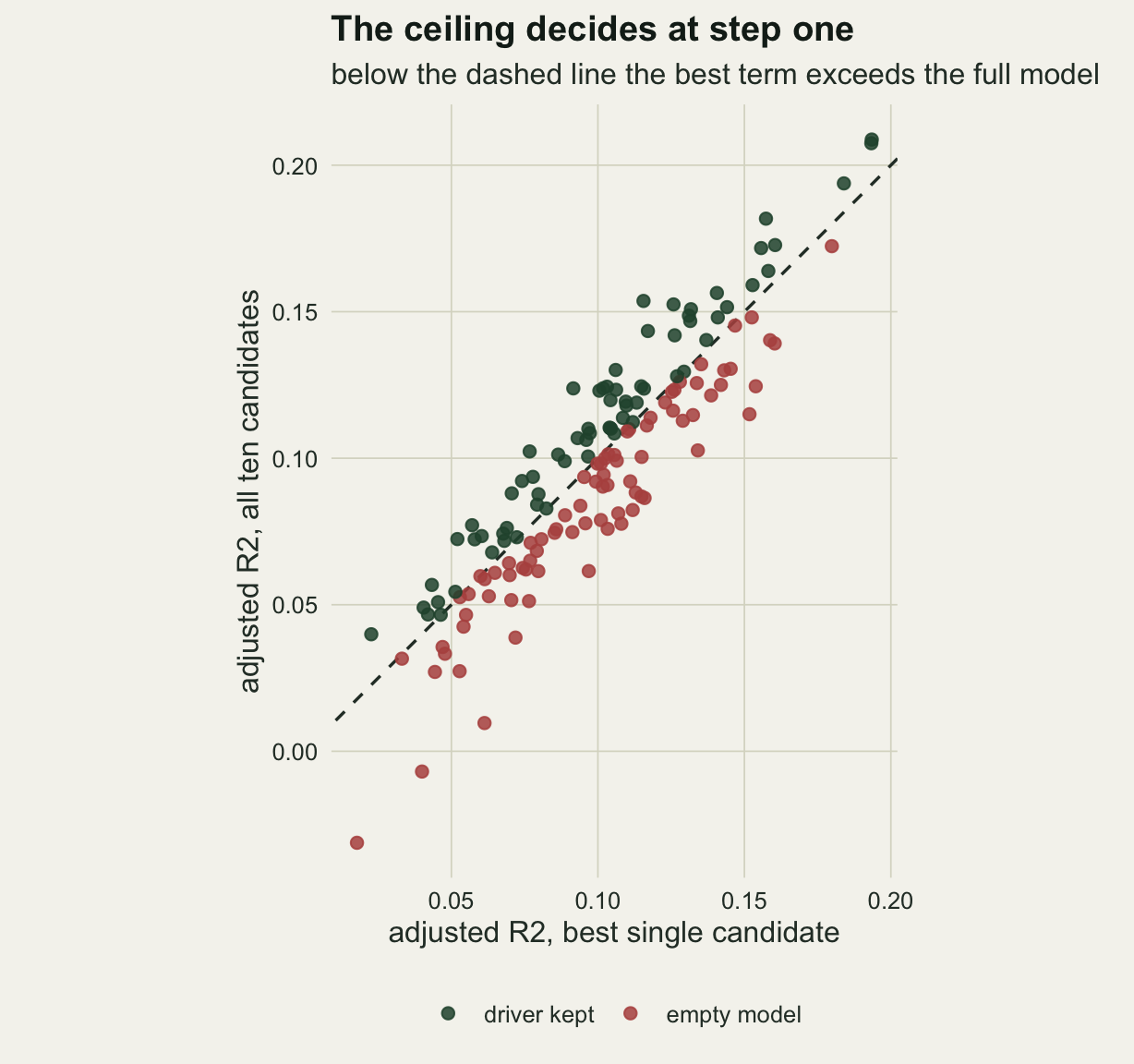
How close the closed form is
The pf() value is exact for one Gaussian response. A community table is thirty responses at once, and the pseudo-F is a ratio of sums over species. Sums over many partly independent species are less variable than one species on its own, so the ratio clusters more tightly around one and the chance that it falls below one should sit between one half and the single response value. Both halves of that argument can be checked.
p_cf50  <- pf(1, n_cand - 1, n_site - n_cand - 1)
p_cf120 <- pf(1, 5 - 1, 120 - 5 - 1)

n_gauss <- 4000
set.seed(2605)
f_gauss <- replicate(n_gauss, {
  x_mat <- matrix(rnorm(n_site * n_cand), n_site, n_cand)
  y_vec <- 0.8 * x_mat[, 1] + rnorm(n_site)
  yc <- matrix(y_vec - mean(y_vec)); ss <- sum(yc^2)
  r2_b <- r2_hand(yc, ss, x_mat[, 1, drop = FALSE])
  r2_a <- r2_hand(yc, ss, x_mat)
  ((r2_a - r2_b) / (n_cand - 1)) / ((1 - r2_a) / (n_site - n_cand - 1))
})
rate_gauss <- mean(f_gauss < 1); se_gauss <- mc_se(rate_gauss, n_gauss)

ceiling_only <- function(n_site, n_cand, slope_sd) {
  d <- make_meadows(n_site, n_cand, slope_sd)
  yc <- scale(as.matrix(d$hel), scale = FALSE); ss <- sum(yc^2)
  r2_one <- vapply(seq_len(n_cand),
                   function(k) r2_hand(yc, ss, d$env[, k, drop = FALSE]), 0)
  r2_all <- r2_hand(yc, ss, d$env)
  c(ceil = adj_r2(max(r2_one), n_site, 1) > adj_r2(r2_all, n_site, n_cand),
    best_true = which.max(r2_one) == 1,
    f_rest = ((r2_all - max(r2_one)) / (n_cand - 1)) /
             ((1 - r2_all) / (n_site - n_cand - 1)))
}
slope_grid <- c(0.25, 0.5, 1.0)
n_sweep <- 600
set.seed(2606)
sweep_tab <- do.call(rbind, lapply(list(c(50, 10), c(120, 5)), function(dz) {
  do.call(rbind, lapply(slope_grid, function(s) {
    r <- replicate(n_sweep, ceiling_only(dz[1], dz[2], s))
    data.frame(n_site = dz[1], n_cand = dz[2], slope = s,
               rate = mean(r["ceil", ]), best_true = mean(r["best_true", ]),
               sd_f = sd(r["f_rest", ]))
  }))
}))
sweep_tab$se <- mc_se(sweep_tab$rate, n_sweep)
sw50  <- sweep_tab[sweep_tab$n_site == 50, ]
sw120 <- sweep_tab[sweep_tab$n_site == 120, ]
sd_gauss <- sd(f_gauss)
sw_pool <- c(mean(sw50$rate), mean(sw120$rate))
sw_pool_se <- sqrt(c(sum(sw50$se^2), sum(sw120$se^2))) / 3
z_real <- (sw_pool - c(rate_empty, big_empty)) /
  sqrt(sw_pool_se^2 + c(se_empty, mc_se(big_empty, n_side))^2)
For one Gaussian response the simulated rate is 0.539 against the closed form 0.544, a difference of 0.6 Monte Carlo standard errors; that part is arithmetic, and it is reproduced, not found.
For the Hellinger community the ceiling refused the driver in 0.522, 0.530 and 0.515 of datasets as the species slope standard deviation went from 0.25 to 0.5 to 1.0, each from 600 datasets with a standard error near 0.020. With 120 plots and five candidates the rates were 0.520, 0.530 and 0.525, against a closed form of 0.589. The spread of the pseudo-F confirms the mechanism: its standard deviation over the community datasets at fifty plots is 0.12 on average across the three slopes, against 0.56 for the single Gaussian response.
So pf(1, P - 1, n - P - 1) is an upper guide, and the community rate sits between it and one half. A stronger driver does not help. At fifty plots the driver was the best single candidate in 96, 100 and 100 per cent of datasets at the three slopes, and the rate does not follow the strength, because both adjusted R2 values rise together. The two diamonds in the figure are ordiR2step() itself at a slope of 0.4, from the smaller simulations above; they differ from the mean of the three sweep rates for their design by 0.4 and 0.1 standard errors of the difference, which is no difference worth reading.
sweep_tab$design <- factor(sprintf("%d plots, %d candidates", sweep_tab$n_site,
                                   sweep_tab$n_cand),
                           levels = c("50 plots, 10 candidates", "120 plots, 5 candidates"))
cf_df <- data.frame(design = levels(sweep_tab$design), cf = c(p_cf50, p_cf120))
cf_df$design <- factor(cf_df$design, levels = levels(sweep_tab$design))
real_df <- data.frame(design = factor(levels(sweep_tab$design),
                                      levels = levels(sweep_tab$design)),
                      slope = slope_one + c(-0.03, 0.03),
                      rate = c(rate_empty, big_empty),
                      se = c(se_empty, mc_se(big_empty, n_side)))
ggplot(sweep_tab, aes(slope, rate, colour = design)) +
  geom_hline(yintercept = 0.5, colour = te_body, linetype = "dotted", linewidth = 0.5) +
  geom_hline(data = cf_df, aes(yintercept = cf, colour = design),
             linetype = "dashed", linewidth = 0.6) +
  geom_errorbar(aes(ymin = rate - 2 * se, ymax = rate + 2 * se), width = 0.03,
                linewidth = 0.4) +
  geom_line(linewidth = 0.9) + geom_point(size = 2.4) +
  geom_errorbar(data = real_df, aes(ymin = rate - 2 * se, ymax = rate + 2 * se),
                width = 0.03, linewidth = 0.4) +
  geom_point(data = real_df, shape = 23, size = 3, fill = te_paper, stroke = 1) +
  scale_colour_manual(values = c(te_forest, te_gold), name = NULL) +
  scale_y_continuous(limits = c(0.25, 0.75)) +
  labs(x = "species slope SD of the driver (log scale units)",
       y = "share of datasets, driver refused",
       title = "About a coin toss, whatever the driver's strength",
       subtitle = "dotted: one half; bars: two Monte Carlo SE") +
  theme_datasheet() + theme(legend.position = "bottom")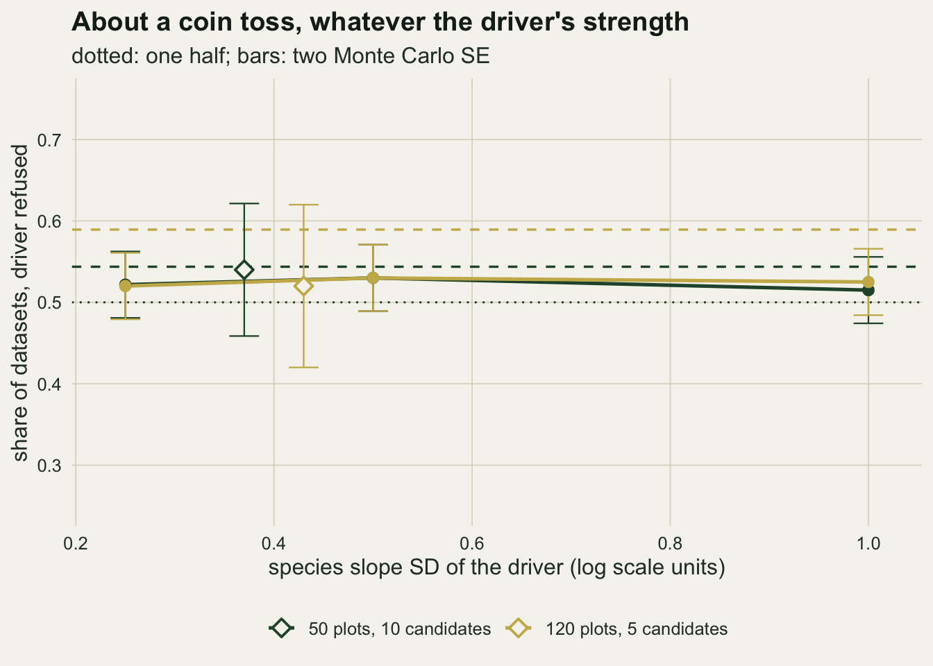
The same rule protects under the null
The ceiling is not a defect. Run the same selection on meadows where none of the ten variables matters and it is the thing that keeps noise out, because there the full model’s adjusted R2 is an estimate of zero, and the best of ten noise candidates, picked for being the best, beats it most of the time.
any_noise <- function(sim, key) mean(sim[key, ] > 0)
null_step  <- any_noise(sim_null, "step_noise")
null_r2s   <- any_noise(sim_null, "r2s_noise")
null_gate  <- mean(sim_null["glob", ] == 1)
null_blan  <- mean(sim_null["glob", ] == 1 & sim_null["r2s_noise", ] > 0)
null_nocap <- any_noise(sim_null, "nocap_noise")
null_ceil  <- mean(sim_null["adj_best", ] > sim_null["adj_all", ])
null_empty <- mean(sim_null["r2s_noise", ] == 0)
step_noise_mean <- mean(sim_null["step_noise", ])
one_blan_keep  <- mean(sim_one["glob", ] == 1 & sim_one["r2s_true", ] == 1)
one_nocap_keep <- mean(sim_one["nocap_true", ] == 1)
one_step_noise <- mean(sim_one["step_noise", ] > 0)
one_r2s_noise  <- mean(sim_one["r2s_noise", ] > 0)
one_nocap_noise <- mean(sim_one["nocap_noise", ] > 0)
Over 150 null datasets ordiR2step() returned the empty model 83.3 per cent of the time, and the ceiling alone was enough in 71.3 per cent. It let at least one noise variable into the model in 16.7 per cent of datasets (Monte Carlo standard error 3.0 points). ordistep() with its default direction did so in 39.3 per cent (standard error 4.0), keeping 0.51 noise terms per dataset on average. The permutation P value of the best of ten candidates is not a P value for a prespecified term, and ten looks at five per cent add up, which is the inflated Type I error Blanchet and colleagues set out to prevent.
That is the asymmetry the post turns on, and it needs both rates side by side. The rule that returned the empty model in 83.3 per cent of null datasets, which is what an analyst wants there, returned it in 54.0 per cent of one driver datasets, where the driver was real and ordistep() found it 100 per cent of the time. The ceiling cannot tell the two situations apart, because in both it compares two estimates of the same population quantity: zero in one case, the driver’s share in the other.
With three drivers, the last one is at risk
The coin toss is not special to a lone driver. With three real drivers of equal strength, the first two are protected in the population: as long as another real driver is still outside the model, the full model explains more than the candidate model, and the ceiling sits above it. In a sample that protection is not complete, as the counts below show. The third is the lone driver again. Adding it makes the current model and the full model the same in the population, and the refusal happens when the pseudo-F of the seven noise candidates given the three drivers is below one.
three_kept <- table(factor(sim_three["r2s_true", ], levels = 0:3))
three_all  <- mean(sim_three["r2s_true", ] == 3)
three_flast <- mean(sim_three["f_last", ] < 1)
three_agree <- mean((sim_three["r2s_true", ] < 3) == (sim_three["f_last", ] < 1))
three_mean_r2s   <- mean(sim_three["r2s_true", ])
three_mean_nocap <- mean(sim_three["nocap_true", ])
p_cf_three <- pf(1, n_cand - 3, n_site - n_cand - 1)
three_one  <- sim_three["r2s_true", ] == 1
three_one_ceil <- sum(three_one & sim_three["stop_why", ] == 1 &
                      sim_three["next_true", ] == 1)
three_kept
 0  1  2  3
 0  3 52 45
Over 100 three driver datasets ordiR2step() kept at least two drivers in 97 per cent, all three in 45 per cent and exactly two in 52 per cent, 2.42 drivers on average. A single driver was kept in 3 datasets and none in 0; in 3 of those 3 the selection stopped at the ceiling, and the candidate it refused was a real driver. There the second driver met the ceiling while the third was still outside: the population argument protects it, and a sample of fifty plots does not always. The pseudo-F of the noise block given the true drivers fell below one in 54 per cent of datasets, the single response closed form for that block is 0.554, and whether that F was below one predicted whether a driver was lost in 99 per cent of datasets. The remainder is the order of entry and the permutation test, which the F condition does not see.
Switching the ceiling off is a trade
Blanchet and colleagues’ full recipe has two steps: test the global model with every candidate first, and only if that test is significant, run the forward selection with both stopping criteria. ordiR2step() carries the second step but not the first, so the recipe needs one anova() call before it. The tempting repair for the lone driver is to keep the global test and drop the ceiling with R2scope = FALSE, so that selection stops on the P value (or when no candidate raises adjusted R2 at all).
rate_row <- function(sim, n, scen, has_step) {
  mk <- function(proc, true_key, noise_key, gate) {
    keep_ok <- if (gate) sim["glob", ] == 1 else rep(TRUE, ncol(sim))
    tr <- sim[true_key, ] * keep_ok; nz <- sim[noise_key, ] * keep_ok
    data.frame(scenario = scen, procedure = proc,
               noise = mean(nz), noise_se = sd(nz) / sqrt(n),
               drivers = mean(tr), drivers_se = sd(tr) / sqrt(n))
  }
  out <- rbind(mk("ordiR2step, defaults", "r2s_true", "r2s_noise", FALSE),
               mk("global test, then ordiR2step", "r2s_true", "r2s_noise", TRUE),
               mk("global test, then R2scope = FALSE", "nocap_true", "nocap_noise", FALSE))
  if (has_step) out <- rbind(mk("ordistep, defaults", "step_true", "step_noise", FALSE), out)
  out
}
proc_lev <- c("ordistep, defaults", "ordiR2step, defaults",
              "global test, then ordiR2step", "global test, then R2scope = FALSE")
scen_lev <- c("no driver", "one driver", "three drivers")
trade_tab <- rbind(rate_row(sim_null, n_rep, scen_lev[1], TRUE),
                   rate_row(sim_one, n_rep, scen_lev[2], TRUE),
                   rate_row(sim_three, n_side, scen_lev[3], FALSE))
trade_tab$procedure <- factor(trade_tab$procedure, levels = proc_lev)
trade_tab$scenario  <- factor(trade_tab$scenario, levels = scen_lev)
tt <- function(scen, proc, col) trade_tab[trade_tab$scenario == scen &
                                          trade_tab$procedure == proc, col]
In the one driver design the global test was significant in 95 per cent of datasets. The full recipe, global test then ordiR2step() with its ceiling, kept moisture in 46 per cent; with the ceiling switched off it kept moisture in 95 per cent. The price is paid in noise. A noise variable entered alongside moisture in 24 per cent of one driver datasets without the ceiling, against 9 per cent for ordiR2step() with its ceiling and 27 per cent for ordistep(). With three drivers, the uncapped route kept 2.95 drivers on average against 2.42, and 0.28 noise terms per dataset against 0.12.
Under the null the global test does most of the work for either version: it was significant in 3.3 per cent of null datasets, and the share with any noise term was 2.0 per cent for the full recipe and 2.7 per cent without the ceiling. The gate protects the null; the ceiling, once past the gate, mostly decides how many noise terms ride along with real drivers, and whether a lone real driver survives.
proc_cols   <- c(te_ink, te_rust, te_gold, te_forest)
proc_shapes <- c(16, 17, 15, 18)
names(proc_cols) <- proc_lev; names(proc_shapes) <- proc_lev
trade_tab <- trade_tab[!is.na(trade_tab$noise), ]
trade_tab$xpos <- as.numeric(trade_tab$scenario) +
  (as.numeric(trade_tab$procedure) - 2.5) * 0.17
trade_plot <- function(dat, yvar, yse, ylab, ttl, ymax, xlo) {
  ggplot(dat, aes(xpos, .data[[yvar]], colour = procedure, shape = procedure)) +
    geom_errorbar(aes(ymin = .data[[yvar]] - 2 * .data[[yse]],
                      ymax = .data[[yvar]] + 2 * .data[[yse]]),
                  width = 0.08, linewidth = 0.5) +
    geom_point(size = 2.8) +
    scale_colour_manual(values = proc_cols, name = NULL, drop = FALSE) +
    scale_shape_manual(values = proc_shapes, name = NULL, drop = FALSE) +
    scale_x_continuous(breaks = seq_along(scen_lev), labels = scen_lev,
                       limits = c(xlo, 3.5)) +
    coord_cartesian(ylim = c(0, ymax)) +
    guides(colour = guide_legend(nrow = 2), shape = guide_legend(nrow = 2)) +
    labs(x = NULL, y = ylab, title = ttl) +
    theme_datasheet() + theme(panel.grid.major.x = element_blank())
}
p_drv   <- trade_plot(trade_tab[trade_tab$scenario != scen_lev[1], ], "drivers",
                      "drivers_se", "real drivers kept, mean", "Real drivers", 3.05, 1.5)
p_noise <- trade_plot(trade_tab, "noise", "noise_se", "noise variables kept, mean",
                      "Noise variables", max(trade_tab$noise + 2 * trade_tab$noise_se), 0.5)
p_drv + p_noise + plot_layout(guides = "collect") +
  plot_annotation(theme = theme_datasheet()) & theme(legend.position = "bottom")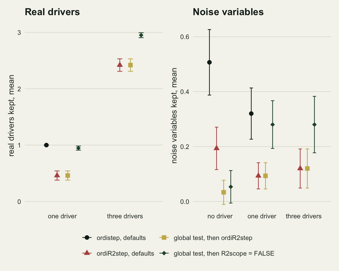
What to report
Name the function and every argument that differs from its default, including the permutation count, and say whether a global test was run first. ordistep() and ordiR2step() answer different questions, and a methods section that says “forward selection in vegan” leaves the reader unable to tell which one, or whether the direction was "both".
When ordiR2step() returns the empty model after a significant global test, report the two adjusted R2 values it compared: the best single candidate’s and the full scope’s. In the worked example the global test gave P = 0.02 with 99 permutations, and the two values were 0.0674 and 0.0515. A reader who sees those numbers knows the empty model came from the ceiling at step one and not from a failed permutation test, and can see how narrow the margin was.
Treat the full scope’s adjusted R2 as what it is, an estimate with its own sampling error that depends on how many candidates were put on the sheet. Adding five more irrelevant variables to the scope moves the ceiling, and with it the selected model. The candidate list is part of the method and belongs in the report.
If the ceiling is switched off to rescue a driver, say so, and say that it was decided after seeing the empty model. On the numbers above that choice keeps a lone driver more often and admits noise variables more often; neither version is free, and the choice made after the fact is itself a data dependent step that the permutation P values do not account for. Whittingham and colleagues (2006) set out the general case against reading stepwise selections as if the model had been fixed in advance, and nothing here repeals it.
Honest limits
The candidates are independent standard normals. Field variables are correlated, moisture with clay and elevation, nitrogen with phosphorus, and correlated candidates change both which one is the best single term and how the noise block’s pseudo-F behaves. The algebra of the ceiling does not change, but the rates measured here should not be carried to a correlated candidate list without rerunning the code on it.
The species respond log linearly to each driver, and the ordination is a linear RDA on Hellinger transformed counts. Unimodal responses along a long gradient, other transformations and distance-based RDA were not simulated. The ceiling comparison is the same for capscale() and dbrda() models when adjusted R2 is available, but the rates were not measured for them.
Every permutation test here used 99 permutations rather than the defaults, so the smallest attainable P value is one in a hundred. That affects the P value criterion and the global test, not the ceiling, which involves no permutation for rda(). Each simulated meadow is drawn from its own seed, fixed in advance, before any test runs on it, so the meadows, their adjusted R2 values and the ceiling comparisons reproduce whatever vegan is installed. The permutations themselves belong to the installed vegan and permute: a version that draws or uses them differently gives different P values, and every rate that involves a permutation test can then move within its Monte Carlo error.
Replication was fixed before running: 150 datasets for the null and one driver designs, 100 for the three driver and larger designs, and 600 per cell for the ceiling sweep, which computes the ceiling condition by hand rather than calling ordiR2step(). That shortcut is justified by the per dataset agreement shown above, not assumed. ordistep() was left out of the three driver design because its drop and add permutations are the expensive part of the whole page; how many drivers it keeps there is not measured.
The one driver and three driver designs put all the signal in named variables and none anywhere else. A community with many weak drivers, some measured and some not, sits between the designs simulated here, and where it sits decides how often a real variable is the last one in and exposed to the coin toss.
References
Blanchet FG, Legendre P, Borcard D 2008 Ecology 89(9):2623-2632 (10.1890/07-0986.1)
Peres-Neto PR, Legendre P, Dray S, Borcard D 2006 Ecology 87(10):2614-2625 (10.1890/0012-9658(2006)87[2614:VPOSDM]2.0.CO;2)
Legendre P, Gallagher ED 2001 Oecologia 129(2):271-280 (10.1007/s004420100716)
Whittingham MJ, Stephens PA, Bradbury RB, Freckleton RP 2006 Journal of Animal Ecology 75(5):1182-1189 (10.1111/j.1365-2656.2006.01141.x)