---
title: "Contrasts and post-hoc comparisons in R"
description: "After a significant ANOVA, which groups differ? Treatment versus sum coding, planned and trend contrasts, Tukey HSD, and correcting pairwise tests."
date: "2026-06-26 11:00"
categories: [R, linear models, ANOVA, multiple comparisons, ecology tutorial]
image: thumbnail.png
image-alt: "A forest plot of pairwise differences in mean biomass between nitrogen treatments, with confidence intervals; five pairs are significant and one crosses zero."
---
A one-way ANOVA tells you that some group means differ, and nothing more. The [previous post](../linear-models-t-test-anova/) showed that the test is just a linear model with a factor, and that a significant F leaves two questions open. First, the coefficients you get depend on how the factor is coded, so you need to choose a coding that answers the comparison you care about. Second, once you start asking which specific groups differ, you are running several tests at once, and the chance of a false positive grows with each one. This post covers both: contrast coding, planned and trend contrasts, and post-hoc pairwise comparisons with a multiplicity correction.
The data is a nitrogen addition experiment: aboveground biomass measured on plots at four nitrogen levels, fifteen plots each. Fertilisation raises biomass, which is one of the better-documented effects in grassland ecology.
```{r}
#| include: false
library(ggplot2)
library(dplyr)
paper <- "#f5f4ee"; ink <- "#16241d"; body <- "#2c3a31"
forest <- "#275139"; label <- "#46604a"; faint <- "#5d6b61"; line <- "#dad9ca"
n_cols <- c(Control = "#c9b458", Low = "#7a9a4e", Medium = "#3f7d4e", High = "#1d5b4e")
base_theme <- theme_minimal(base_size = 13) +
theme(plot.background = element_rect(fill = paper, colour = NA),
panel.background = element_rect(fill = paper, colour = NA),
panel.grid.minor = element_blank(),
panel.grid.major = element_line(colour = line, linewidth = 0.3),
axis.title = element_text(colour = body),
axis.text = element_text(colour = faint),
legend.position = "none")
```
```{r}
set.seed(116)
ng  <- 15
lev <- c("Control", "Low", "Medium", "High")
nit <- data.frame(
  nitrogen = factor(rep(lev, each = ng), levels = lev),
  biomass  = c(rnorm(ng, 250, 50), rnorm(ng, 320, 50),
               rnorm(ng, 400, 50), rnorm(ng, 430, 50))
)

m <- lm(biomass ~ nitrogen, data = nit)
anova(m)
```
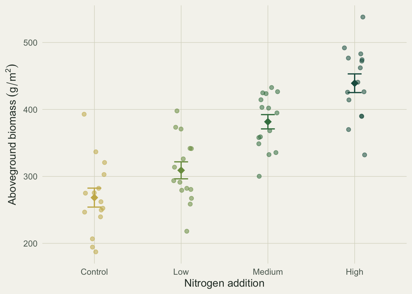
The omnibus F is 34.4 on 3 and 56 degrees of freedom, with a p-value near `9.6e-13`: the four means are not all equal, and nitrogen explains about 65 percent of the variation in biomass. Group means run from 268 g/m^2 in the control to 439 g/m^2 at high nitrogen, with a grand mean of 350.
```{r}
#| fig-cap: "Biomass by nitrogen level. Points are plots, diamonds are means, bars are one standard error."
#| fig-alt: "Jittered biomass for control, low, medium and high nitrogen, rising from about 270 to 440 grams per square metre. Control and low overlap; medium and high are clearly higher."
ggplot(nit, aes(nitrogen, biomass, colour = nitrogen)) +
  geom_jitter(width = 0.12, height = 0, size = 2, alpha = 0.55) +
  stat_summary(fun.data = mean_se, geom = "errorbar", width = 0.16, linewidth = 0.7) +
  stat_summary(fun = mean, geom = "point", size = 4, shape = 18) +
  scale_colour_manual(values = n_cols) +
  labs(x = "Nitrogen addition", y = expression(Aboveground~biomass~(g/m^2))) +
  base_theme
```
## Two ways to code the same factor
The coefficients from `lm` are not the group means; they are contrasts, and which contrasts you see depends on the coding scheme. R uses treatment coding by default, which we met in the previous post: the first level becomes a reference folded into the intercept, and the other coefficients are differences from it.
```{r}
summary(m)$coefficients
```
The intercept, 268, is the control mean. Each other coefficient is the rise above the control: low adds 41 g/m^2, medium adds 113, high adds 171. This is the right coding when one level is a natural baseline, which here it is.
Sum-to-zero coding answers a different question. It makes the intercept the grand mean and each coefficient a deviation from it, with the last level dropped because the deviations sum to zero.
```{r}
m_sum <- lm(biomass ~ nitrogen, data = nit, contrasts = list(nitrogen = contr.sum))
summary(m_sum)$coefficients
```
Now the intercept is 350, the grand mean, and its standard error (6.5) is smaller than the treatment intercept's (12.9), because the grand mean pools all sixty plots while the control mean used only fifteen. The three coefficients are the deviations of control, low and medium from the grand mean (-81, -40, +32); the high deviation is not printed, but it is the negative of their sum, +90, which is exactly high minus the grand mean. The two models describe the same fit: their fitted values are identical to machine precision. Coding changes what the parameters mean, not what the model predicts. Sum coding is the convention behind classical ANOVA tables and is the sensible choice when no level is special, for instance when you later add an interaction and want main effects that are not tied to one reference cell.
## Planned contrasts
A contrast is a weighted combination of group means with weights that sum to zero, and it lets you test a comparison decided in advance rather than fishing through all pairs. Two kinds are worth knowing.
When the factor is ordered, polynomial contrasts split the effect into a linear trend, a quadratic (curvature), a cubic, and so on. Declaring nitrogen ordered makes R fit these automatically.
```{r}
nit$nit_ord <- factor(nit$nitrogen, levels = lev, ordered = TRUE)
summary(lm(biomass ~ nit_ord, data = nit))$coefficients
```
The linear term is large and highly significant (`t = 10.1`), while the quadratic (`p = 0.52`) and cubic (`p = 0.42`) are not: biomass climbs with nitrogen along an essentially straight line over this range, with no detectable bend. A single linear-trend test like this is far more focused, and more powerful, than an omnibus F when a monotone dose response is what you expect.
Any other planned comparison is a contrast vector applied to the group means. Suppose the question is whether adding nitrogen at all changes biomass: control against the average of the three fertilised levels. The weights are `c(1, -1/3, -1/3, -1/3)`, and the estimate, its standard error, and a t test come straight from the group means and the model's residual variance.
```{r}
gm     <- tapply(nit$biomass, nit$nitrogen, mean)
Lvec   <- c(1, -1/3, -1/3, -1/3)
sigma2 <- summary(m)$sigma^2
est    <- sum(Lvec * gm)
se     <- sqrt(sigma2 * sum(Lvec^2 / ng))
c(estimate = est, se = se, t = est / se,
  p = 2 * pt(-abs(est / se), df = m$df.residual))
```
Control biomass sits 108 g/m^2 below the fertilised average (`t = -7.2`, `p` near `1e-09`). Because this is one comparison chosen before seeing the data, it needs no correction: the multiplicity problem only arises when you test many comparisons at once, which is what post-hoc analysis does.
## Post-hoc: which pairs differ?
With no prior hypothesis you may want every pairwise comparison. For four groups that is six tests, and testing six things at the 0.05 level means the chance of at least one false positive is well above 0.05. Tukey's honest significant difference is built for exactly this case: it compares all pairs while holding the family-wise error rate at the stated level, using the distribution of the largest difference among the means.
```{r}
TukeyHSD(aov(biomass ~ nitrogen, data = nit))$nitrogen
```
```{r}
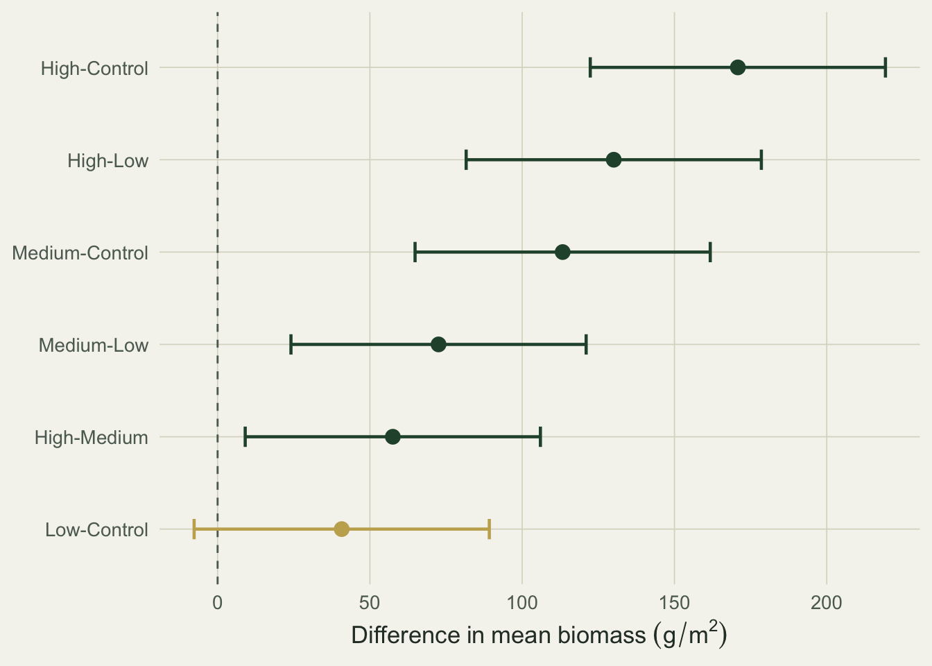
#| fig-cap: "Tukey HSD pairwise differences with family-wise 95 percent intervals. Green intervals exclude zero; the gold one (low versus control) does not."
#| fig-alt: "Forest plot of six pairwise biomass differences with confidence intervals. Five intervals lie entirely above zero and are green; the low-versus-control interval crosses zero and is gold."
td <- as.data.frame(TukeyHSD(aov(biomass ~ nitrogen, data = nit))$nitrogen)
td$pair <- rownames(td)
td$sig  <- factor(td$`p adj` < 0.05, levels = c(TRUE, FALSE))

ggplot(td, aes(diff, reorder(pair, diff), colour = sig)) +
  geom_vline(xintercept = 0, linetype = "dashed", colour = faint, linewidth = 0.5) +
  geom_errorbarh(aes(xmin = lwr, xmax = upr), height = 0.22, linewidth = 0.8) +
  geom_point(size = 3.2) +
  scale_colour_manual(values = c("TRUE" = forest, "FALSE" = "#c4ad5e")) +
  labs(x = expression(Difference~"in"~mean~biomass~(g/m^2)), y = NULL) +
  base_theme
```
Five of the six pairs differ. The exception is low versus control: the difference is 41 g/m^2 but the family-wise interval runs from -8 to 89 and includes zero, so the lowest dose is not separable from the control. Everything from medium upward is.
`pairwise.t.test` runs the same comparisons and lets you choose the correction explicitly. The choice matters most at the boundary.
```{r}
sapply(c("none", "bonferroni", "holm", "BH"),
       function(a) pairwise.t.test(nit$biomass, nit$nitrogen,
                                   p.adjust.method = a)$p.value["Low", "Control"])
```
Low versus control is the borderline case. Unadjusted it is significant (0.03); Holm and Benjamini-Hochberg keep it significant (0.03), Bonferroni does not (0.18), and Tukey called it non-significant too. Four valid procedures, two verdicts. The honest reading is that the lowest dose is right at the edge of detectability, and the label depends on the method, so report the estimate and its interval rather than leaning on a single star.
## Why the correction is not optional
To see what unadjusted pairwise tests cost, simulate the situation where there is genuinely no effect: four groups drawn from one distribution, all six pairwise comparisons run, repeated two thousand times. The family-wise error rate is the fraction of datasets where at least one comparison comes out significant.
```{r}
set.seed(909)
R <- 2000; ng2 <- 12; k <- 4
g  <- factor(rep(seq_len(k), each = ng2))
sims <- replicate(R, {
  y    <- rnorm(ng2 * k)
  praw <- pairwise.t.test(y, g, p.adjust.method = "none")$p.value
  praw <- praw[!is.na(praw)]
  c(none = min(praw),
    bonferroni = min(p.adjust(praw, "bonferroni")),
    holm = min(p.adjust(praw, "holm")))
})
fwer <- rowMeans(sims < 0.05)
round(fwer, 4)
```
```{r}
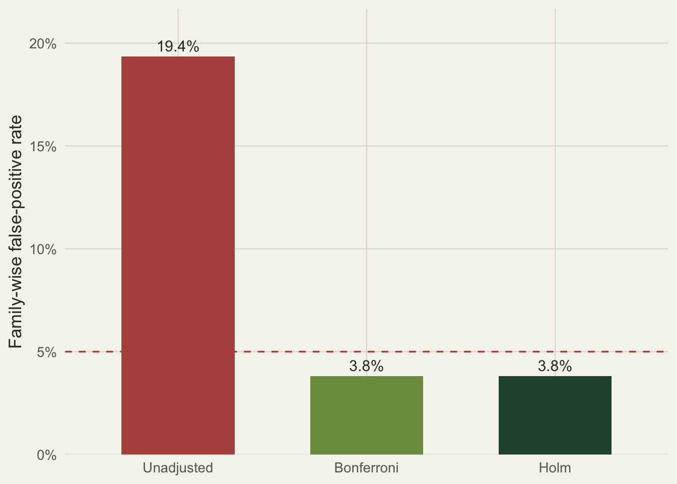
#| fig-cap: "Family-wise false-positive rate under the global null, by correction. The dashed line marks the nominal 5 percent."
#| fig-alt: "Bar chart of family-wise false-positive rates: unadjusted near 19 percent, well above a dashed line at 5 percent; Bonferroni and Holm both near 4 percent, below the line."
fd <- data.frame(method = factor(names(fwer), levels = names(fwer)),
                 rate = as.numeric(fwer))
levels(fd$method) <- c("Unadjusted", "Bonferroni", "Holm")

ggplot(fd, aes(method, rate, fill = method)) +
  geom_col(width = 0.6) +
  geom_hline(yintercept = 0.05, linetype = "dashed", colour = "#b5534e", linewidth = 0.6) +
  geom_text(aes(label = sprintf("%.1f%%", 100 * rate)), vjust = -0.5, colour = body, size = 4) +
  scale_fill_manual(values = c(Unadjusted = "#b5534e", Bonferroni = "#7a9a4e", Holm = "#275139")) +
  scale_y_continuous(expand = expansion(mult = c(0, 0.12)),
                     labels = function(x) paste0(x * 100, "%")) +
  labs(x = NULL, y = "Family-wise false-positive rate") +
  base_theme
```
Without a correction, about one run in five flags a difference that is not there: a 19 percent error rate where 5 percent was intended. Bonferroni and Holm both pull it back below the nominal level (to about 0.04). They give the same family-wise protection here, and that is not a coincidence: family-wise error is controlled by the smallest p-value, and both methods multiply the smallest p by the same factor. Where Holm wins is everywhere else. It penalises the larger p-values less, which is why it kept low-versus-control significant on the real data while Bonferroni did not. Use Holm over Bonferroni by default; use Benjamini-Hochberg when you can tolerate a controlled false discovery rate in exchange for more power across many comparisons.
In day-to-day work the [emmeans package](https://cran.r-project.org/package=emmeans) (Lenth) does all of this in one place: estimated marginal means, any contrast you write down, and the matching adjustment, including for models with covariates and interactions where hand computation gets awkward. Everything above is base R so the machinery is visible, but emmeans is the tool to reach for once you understand what it is doing.
The same logic carries to the multivariate setting. When the response is a whole community rather than one number, the omnibus test is PERMANOVA and the follow-up is pairwise PERMANOVA with the identical multiplicity problem and the identical fixes, which the [pairwise PERMANOVA post](../pairwise-permanova/) works through.
## References
Tukey 1949 Biometrics 5(2):99-114 (10.2307/3001913).
Dunn 1961 Journal of the American Statistical Association 56(293):52-64 (10.1080/01621459.1961.10482090).
Holm 1979 Scandinavian Journal of Statistics 6(2):65-70 (10.2307/4615733).
Benjamini and Hochberg 1995 Journal of the Royal Statistical Society Series B 57(1):289-300 (10.1111/j.2517-6161.1995.tb02031.x).