set.seed(5310)
n<-500; gamma_t<-0.7; sigma_t<-4; tau_t<-6
vx<-vy<-numeric(n)
vx[1]<-rnorm(1,0,sigma_t/sqrt(1-gamma_t^2)); vy[1]<-rnorm(1,0,sigma_t/sqrt(1-gamma_t^2))
for(t in 2:n){ vx[t]<-gamma_t*vx[t-1]+rnorm(1,0,sigma_t); vy[t]<-gamma_t*vy[t-1]+rnorm(1,0,sigma_t) }
px<-cumsum(vx); py<-cumsum(vy); ox<-px+rnorm(n,0,tau_t); oy<-py+rnorm(n,0,tau_t)Checking a state-space movement model
movement ecology
state-space models
model diagnostics
R
ecology tutorial
Check a fitted state-space movement model with one-step-ahead prediction residuals in base R: QQ plots and autocorrelation reveal what a misspecified model hides.
A state-space model can converge, return sensible parameters, and still be wrong. The three earlier posts in this series fitted movement models and trusted the output; this one asks how to tell whether that trust is warranted. The tool is the same by-product the Kalman filter produced all along: the one-step-ahead prediction residual, or innovation. If the model is correct, the standardised innovations are independent standard normal draws. Any departure, especially leftover autocorrelation, is the fingerprint of a misspecified model. We show that a plausible but wrong model passes the obvious marginal check and fails only the one that matters.
Innovations as residuals
At each step the Kalman filter predicts the next observation before seeing it. The gap between prediction and observation is the innovation \(v_t\), and the filter also returns its variance \(F_t\). Dividing gives the standardised innovation \(v_t / \sqrt{F_t}\). Under the true model these are uncorrelated and standard normal, so the same two diagnostics used for any regression apply: a normal quantile plot for the marginal shape, and an autocorrelation function for independence. The autocorrelation check is the sharper of the two, because a wrong dynamic model can still produce roughly normal residuals while leaving them correlated in time.
Two models for one track
We simulate a track with genuine directional persistence and observation error, then fit two models. The correct one is the correlated random walk state-space model of the first post, with a velocity that persists. The wrong one is a plain random-walk-on-position model with observation error but no velocity term, so it cannot represent momentum. Both filters return standardised innovations.
## correct: correlated random walk (position + velocity), returns standardised innovations
kf_crw<-function(y,g,s2,h2){
  n<-length(y); Tm<-matrix(c(1,0,g,g),2,2); Q<-s2*matrix(c(1,1,1,1),2,2); Z<-matrix(c(1,0),1,2)
  a<-c(y[1],0); P<-matrix(c(h2,0,0,s2/(1-g^2)),2,2); ll<-0; r<-rep(NA,n)
  for(t in 2:n){ ap<-as.vector(Tm%*%a); Pp<-Tm%*%P%*%t(Tm)+Q
    v<-y[t]-as.vector(Z%*%ap); Ft<-as.vector(Z%*%Pp%*%t(Z))+h2; K<-as.vector(Pp%*%t(Z))/Ft
    a<-ap+K*v; P<-Pp-(K%*%Z)%*%Pp; ll<-ll-0.5*(log(2*pi)+log(Ft)+v^2/Ft); r[t]<-v/sqrt(Ft) }
  list(ll=ll, r=r) }
## wrong: random walk on position, no persistence
kf_rw<-function(y,s2,h2){
  n<-length(y); ll<-0; r<-rep(NA,n); a<-y[1]; P<-h2
  for(t in 2:n){ ap<-a; Pp<-P+s2; v<-y[t]-ap; Ft<-Pp+h2; K<-Pp/Ft
    a<-ap+K*v; P<-Pp-K*Pp; ll<-ll-0.5*(log(2*pi)+log(Ft)+v^2/Ft); r[t]<-v/sqrt(Ft) }
  list(ll=ll, r=r) }

nA<-function(p){g<-plogis(p[1]);s2<-exp(p[2]);h2<-exp(p[3]);-(kf_crw(ox,g,s2,h2)$ll+kf_crw(oy,g,s2,h2)$ll)}
fA<-optim(c(0,log(16),log(16)),nA,method="Nelder-Mead",control=list(reltol=1e-10,maxit=3000))
gA<-plogis(fA$par[1]);s2A<-exp(fA$par[2]);h2A<-exp(fA$par[3])
nB<-function(p){s2<-exp(p[1]);h2<-exp(p[2]);-(kf_rw(ox,s2,h2)$ll+kf_rw(oy,s2,h2)$ll)}
fB<-optim(c(log(16),log(16)),nB,method="Nelder-Mead",control=list(reltol=1e-10,maxit=3000))
s2B<-exp(fB$par[1]);h2B<-exp(fB$par[2])
aicA<-2*3+2*fA$value; aicB<-2*2+2*fB$value
c(gamma=round(gA,3), sigma=round(sqrt(s2A),2), tau=round(sqrt(h2A),2), dAIC=round(aicB-aicA,1))
gamma sigma tau dAIC
0.757 3.630 6.250 66.100 Model selection already prefers the correct model: the correlated random walk fits with persistence 0.757, and beats the random-walk model by 66.1 AIC units. But AIC only ranks; it does not tell us whether even the winner is adequate. For that we turn to the residuals.
rAx<-kf_crw(ox,gA,s2A,h2A)$r[-1]; rAy<-kf_crw(oy,gA,s2A,h2A)$r[-1]
rBx<-kf_rw(ox,s2B,h2B)$r[-1];     rBy<-kf_rw(oy,s2B,h2B)$r[-1]
rApool<-c(rAx,rAy); rBpool<-c(rBx,rBy)
qqcor<-function(r){q<-qqnorm(r,plot.it=FALSE); cor(q$x,q$y)}
acfA<-acf(rAx,plot=FALSE,lag.max=18); acfB<-acf(rBx,plot=FALSE,lag.max=18)
bnd<-1.96/sqrt(length(rBx))
lbA<-mean(c(Box.test(rAx,10,"Ljung-Box")$p.value, Box.test(rAy,10,"Ljung-Box")$p.value))
lbB<-mean(c(Box.test(rBx,10,"Ljung-Box")$p.value, Box.test(rBy,10,"Ljung-Box")$p.value))
qq_A<-qqcor(rApool); qq_B<-qqcor(rBpool)
a234<-round(acfB$acf[3:5,1,1],3)   # lags 2, 3, 4 of the wrong model
c(qq_correct=round(qq_A,4), qq_wrong=round(qq_B,4), LB_correct=round(lbA,3), LB_wrong=signif(lbB,3))
qq_correct qq_wrong LB_correct LB_wrong
0.999600 0.999600 0.716000 0.000142 The marginal check misses it
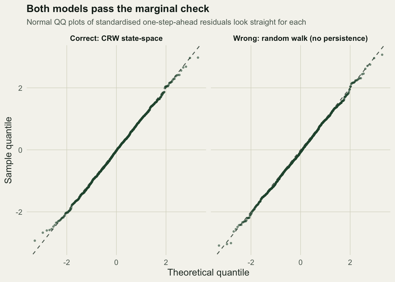
The normal quantile plot looks at the shape of the residual distribution, ignoring order. Both models pass: the quantile correlation is 0.9996 for the correct model and 0.9996 for the wrong one, essentially indistinguishable. A practitioner who stops here would accept the wrong model.
The autocorrelation check catches it
Independence is where the wrong model breaks. Because it cannot represent directional persistence, the animal keeps moving in the same direction for several steps and the one-step prediction errors stay correlated. The correlation is masked at lag one by the differencing of observation noise, but it shows plainly at the next few lags.
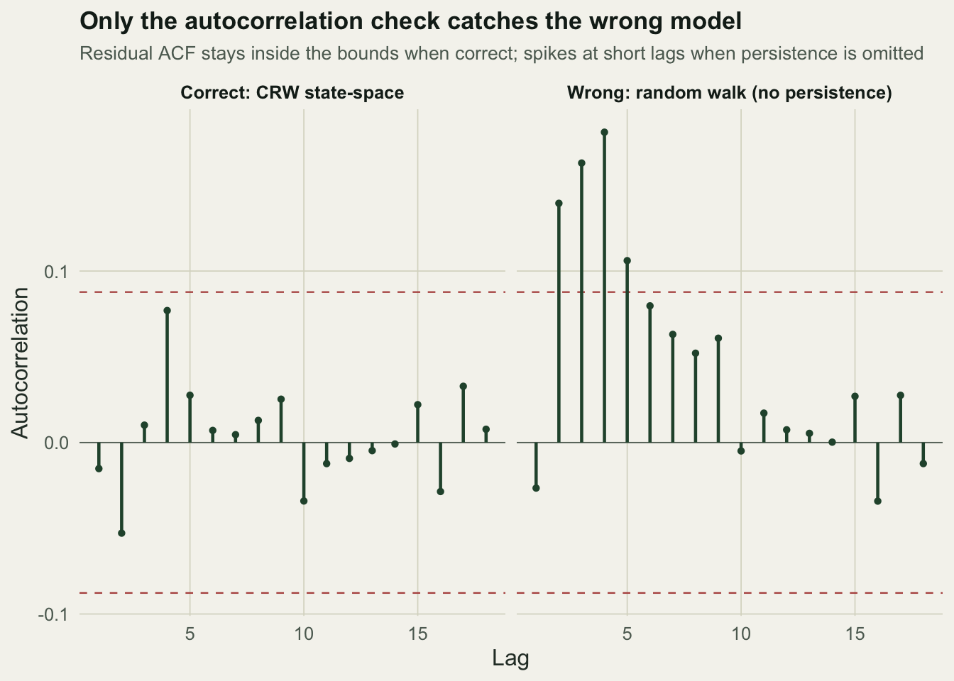
The correct model’s residual autocorrelations all sit inside the 0.088 bound, and a portmanteau test over the first ten lags is comfortably non-significant, with a p-value of 0.716. The wrong model tells a different story: its autocorrelations at lags two, three, and four are 0.14, 0.163, and 0.181, all beyond the bound, and the same portmanteau test returns a p-value of 1.42^{-4}. The residual autocorrelation, not the quantile plot, is what exposes the misspecification.
The general lesson
This mirrors the pseudo-residual check for hidden Markov movement models: there too, a model that omits structure leaves autocorrelation in its residuals while the marginal fit looks fine. The habit worth keeping is to judge a fitted state-space model by its one-step-ahead residuals, and to lead with the autocorrelation function. A model can match the marginal distribution of the data and still get the dynamics wrong, and only the independence check will tell you.
References
Durbin and Koopman 2012. Time Series Analysis by State Space Methods, 2nd edn. ISBN 978-0-19-964117-8
Auger-Methe, Newman, Cole, Empacher, Gryba, King, Leos-Barajas, Mills Flemming, Nielsen, Petris and Thomas 2021. Ecological Monographs 91(4):e01470 (10.1002/ecm.1470)
Jonsen, Flemming and Myers 2005. Ecology 86(11):2874-2880 (10.1890/04-1852)
Kalman 1960. Journal of Basic Engineering 82(1):35-45 (10.1115/1.3662552)
Zucchini, MacDonald and Langrock 2016. Hidden Markov Models for Time Series: An Introduction Using R, 2nd edn. ISBN 978-1-4822-5383-2