Bayesian state-space movement

Recover a latent movement path from noisy positions in R: forward-filter backward-sample, conjugate Gibbs updates, and the process-versus-observation noise trade-off.

A GPS or telemetry track is the true path plus measurement error, and the error does real damage. Join the raw fixes with straight lines and the total distance travelled comes out far too long, because every wobble in the observation adds spurious back-and-forth. Turning angles get randomised the same way. The quantities movement ecologists want, path length, speed, tortuosity, are all corrupted by treating the observations as the truth.

A state-space model separates the animal’s latent position from the noisy fix. The frequentist version runs a Kalman filter and maximises the likelihood for point estimates of the movement parameters. Here we do it the Bayesian way, and the payoff is twofold: the latent path comes with a credible band, and the notoriously entangled process and observation variances show their dependence honestly as a joint posterior rather than a pair of point estimates.

The model

The animal moves as a correlated random walk. Its state is position and velocity, and the velocity carries momentum: each step’s velocity is gamma times the last plus Gaussian process noise with standard deviation sigma. Position accumulates velocity. We observe position with Gaussian error of standard deviation tau. Writing the state as a two-vector, the whole thing is linear and Gaussian, which is what lets us sample the entire latent path in one block.

Simulating a noisy track

library(MASS)
set.seed(6142)
n <- 200L
gamma.true <- 0.7; sig.true <- 4; tau.true <- 6   # persistence, process SD, obs SD
x <- numeric(n); v <- numeric(n)
x[1] <- 0; v[1] <- rnorm(1, 0, sig.true / sqrt(1 - gamma.true^2))
for (t in 2:n) {
  x[t] <- x[t-1] + v[t-1]
  v[t] <- gamma.true * v[t-1] + rnorm(1, 0, sig.true)
}
y <- x + rnorm(n, 0, tau.true)                     # noisy observations

The naive path length joins the raw fixes; the true path length joins the latent positions.

path.true <- sum(abs(diff(x)))
path.naive <- sum(abs(diff(y)))

The observations imply a path of 1582 units against a true 1016, an inflation of 1.56 times. That extra distance is pure measurement noise, and it is exactly the kind of bias that inflates estimated energy budgets and home ranges.

Forward-filter backward-sample

The heart of the sampler is a routine that draws the whole latent path at once. It runs a Kalman filter forward to get the filtered mean and covariance at each time, then walks backward, sampling each state from its conditional given the state just sampled after it. For a linear-Gaussian model this returns an exact draw from the joint posterior of the path, which mixes far better than updating one time point at a time.

Hm <- matrix(c(1, 0), 1, 2)                        # observe position only
ffbs <- function(y, gamma, sig2, tau2) {
  n <- length(y)
  A <- matrix(c(1, 0, 1, gamma), 2, 2)             # state transition
  Q <- matrix(c(0, 0, 0, sig2), 2, 2)              # process noise on velocity
  mp <- vector("list", n); Pp <- vector("list", n) # predicted moments
  mf <- vector("list", n); Pf <- vector("list", n) # filtered moments
  m0 <- c(y[1], 0); P0 <- diag(c(100, 100))
  for (t in 1:n) {
    if (t == 1) { mpred <- m0; Ppred <- P0 } else {
      mpred <- A %*% mf[[t-1]]; Ppred <- A %*% Pf[[t-1]] %*% t(A) + Q
    }
    mp[[t]] <- mpred; Pp[[t]] <- Ppred
    S <- Hm %*% Ppred %*% t(Hm) + tau2
    K <- Ppred %*% t(Hm) / as.numeric(S)
    mf[[t]] <- mpred + K %*% (y[t] - Hm %*% mpred)
    Pf[[t]] <- (diag(2) - K %*% Hm) %*% Ppred
    Pf[[t]] <- (Pf[[t]] + t(Pf[[t]])) / 2           # keep symmetric
  }
  s <- matrix(0, n, 2)
  s[n, ] <- mvrnorm(1, mf[[n]], Pf[[n]])
  for (t in (n-1):1) {
    J <- Pf[[t]] %*% t(A) %*% solve(Pp[[t+1]])
    mb <- mf[[t]] + J %*% (s[t+1, ] - mp[[t+1]])
    Pb <- Pf[[t]] - J %*% A %*% Pf[[t]]
    Pb <- (Pb + t(Pb)) / 2
    s[t, ] <- mvrnorm(1, mb, Pb)
  }
  s
}

The Gibbs sampler

Each sweep draws the latent path with FFBS, then updates the three parameters given that path. Both variances are conjugate: an inverse-gamma update from the velocity innovations gives the process variance, and one from the observation residuals gives the observation variance. The persistence gamma is a Gaussian regression of each velocity on the previous one, so it too has a closed-form conjugate update.

n.iter <- 4000L; burn <- 1000L
gam.s <- numeric(n.iter); sig.s <- numeric(n.iter); tau.s <- numeric(n.iter)
path.s <- numeric(n.iter); xstore <- matrix(0, n.iter, n)
gamma <- 0.5; sig2 <- var(diff(y)); tau2 <- var(diff(y)) / 2
for (it in 1:n.iter) {
  s <- ffbs(y, gamma, sig2, tau2)
  xs <- s[, 1]; vs <- s[, 2]
  # process variance from velocity innovations
  eta <- vs[2:n] - gamma * vs[1:(n-1)]
  sig2 <- 1 / rgamma(1, 0.001 + (n-1)/2, 0.001 + sum(eta^2)/2)
  # observation variance from residuals
  r <- y - xs
  tau2 <- 1 / rgamma(1, 0.001 + n/2, 0.001 + sum(r^2)/2)
  # persistence: Gaussian regression v_t on v_{t-1}, prior N(0, 100)
  vprec <- sum(vs[1:(n-1)]^2) / sig2 + 1/100
  vmean <- (sum(vs[1:(n-1)] * vs[2:n]) / sig2) / vprec
  gamma <- rnorm(1, vmean, sqrt(1/vprec))
  gam.s[it] <- gamma; sig.s[it] <- sqrt(sig2); tau.s[it] <- sqrt(tau2)
  path.s[it] <- sum(abs(diff(xs))); xstore[it, ] <- xs
}
keep <- (burn+1):n.iter
gam.p <- gam.s[keep]; sig.p <- sig.s[keep]; tau.p <- tau.s[keep]; path.p <- path.s[keep]

What the posterior recovers

gm <- median(gam.p); gci <- quantile(gam.p, c(.025, .975))
sm <- median(sig.p); sci <- quantile(sig.p, c(.025, .975))
tm <- median(tau.p); tci <- quantile(tau.p, c(.025, .975))
pm <- median(path.p); pci <- quantile(path.p, c(.025, .975))

Persistence has posterior median 0.757 [0.56, 0.88], covering 0.7. Process noise lands at 4.1 [2.92, 6.05] against a true 4, and observation noise at 5.5 [4.57, 6.5] against 6. Path length has posterior median 1062 [977, 1195], covering the true 1016, while the naive 1582 sits far above the upper end of that interval. The model strips the measurement noise back out.

library(ggplot2)
ink <- "#16241d"; forest <- "#275139"; sage <- "#93a87f"; rust <- "#b5534e"; line <- "#dad9ca"
theme_te <- theme_minimal(base_size = 12) +
  theme(panel.grid.minor = element_blank(),
        panel.grid.major = element_line(colour = line, linewidth = 0.3),
        plot.title = element_text(colour = ink, face = "bold", size = 13),
        plot.subtitle = element_text(colour = "#5d6b61", size = 10),
        axis.title = element_text(colour = ink), axis.text = element_text(colour = "#46604a"),
        legend.position = "none")
x.mean <- colMeans(xstore[keep, ])
x.lo <- apply(xstore[keep, ], 2, quantile, 0.025)
x.hi <- apply(xstore[keep, ], 2, quantile, 0.975)
dpath <- data.frame(t = 1:n, truex = x, obsy = y, mx = x.mean, lo = x.lo, hi = x.hi)
ggplot(dpath, aes(t)) +
  geom_ribbon(aes(ymin = lo, ymax = hi), fill = sage, alpha = 0.4) +
  geom_point(aes(y = obsy), colour = "#9aa39a", size = 0.7, alpha = 0.7) +
  geom_line(aes(y = truex), colour = rust, linewidth = 0.7) +
  geom_line(aes(y = mx), colour = forest, linewidth = 0.7) +
  labs(title = "Latent movement path recovered from noisy positions",
       subtitle = "Grey: raw observations. Red: true path. Green with band: posterior path.",
       x = "Time step", y = "Position") + theme_te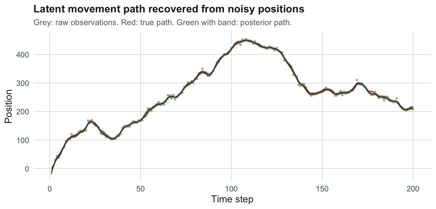

Figure 1: The latent path recovered from noisy observations, with its credible band.

The variances trade off

Process noise and observation noise are hard to tell apart: a jittery track can be a wandering animal seen cleanly, or a steady animal seen poorly. The joint posterior shows that tension directly, as a negative correlation between the two standard deviations.

ggplot(data.frame(sigma = sig.p, tau = tau.p), aes(sigma, tau)) +
  geom_point(colour = forest, alpha = 0.15, size = 0.6) +
  geom_density_2d(colour = ink, linewidth = 0.3, bins = 6) +
  geom_point(aes(x = sig.true, y = tau.true), colour = rust, size = 3) +
  labs(title = "Joint posterior of process and observation noise",
       subtitle = "Negative correlation is the process-versus-observation trade-off. Red: truth.",
       x = "Process SD (sigma)", y = "Observation SD (tau)") + theme_te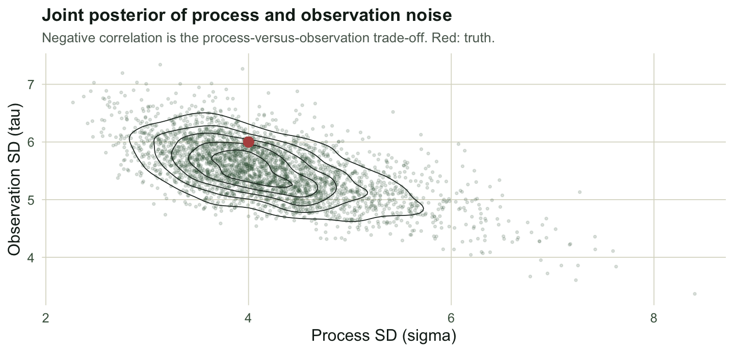

Figure 2: Joint posterior of process and observation noise, showing the trade-off.

The posterior correlation here is about -0.63. A point estimate would hide it, reporting two numbers as if they were independently known. The Kalman-filter treatment discusses why this separation is weakly identified; the Bayesian version simply draws it, and integrating over the dependence is what gives the path band its honest width.

Where this sits

The same block sampler drives any linear-Gaussian state-space model, so it transfers straight to population time series and growth models with observation error. When the movement model is non-linear, as with a state-switching animal, FFBS no longer applies and a particle method or a discrete-state filter takes its place, but the principle holds: sample the latent trajectory, then the parameters. The rest of this Bayesian latent-state series, from survival to abundance, uses the same division of labour with a different hidden quantity.

References

• Kalman 1960, Journal of Basic Engineering 82(1):35-45 (10.1115/1.3662552)
• Carter, Kohn 1994, Biometrika 81(3):541-553 (10.1093/biomet/81.3.541)
• Fruhwirth-Schnatter 1994, Journal of Time Series Analysis 15(2):183-202 (10.1111/j.1467-9892.1994.tb00184.x)
• Jonsen, Flemming, Myers 2005, Ecology 86(11):2874-2880 (10.1890/04-1852)
• Knape 2008, Ecology 89(11):2994-3000 (10.1890/08-0071.1)
• Auger-Methe et al. 2021, Ecological Monographs 91(4):e01470 (10.1002/ecm.1470)

Related tutorials

• State-space models for movement
• Bayesian Cormack-Jolly-Seber survival
• Bayesian N-mixture abundance
• Bayesian closed-population capture-recapture