set.seed(5027)
R <- 150L                 # sites
K <- 4L                   # repeat visits
lambda.true <- 2.8
p.true <- 0.37

N.true <- rpois(R, lambda.true)               # latent site abundance
y <- matrix(0L, R, K)                         # observed counts
for (i in 1:R) y[i, ] <- rbinom(K, N.true[i], p.true)
ymax <- apply(y, 1, max) # naive per-site abundanceBayesian N-mixture abundance
Bayesian statistics
MCMC
abundance
R
ecology tutorial
Fit a Bayesian N-mixture model by hand in R: latent abundance data augmentation, conjugate Gibbs updates, and total abundance the naive maximum count underestimates.
Count the animals at a site on four visits and you never see all of them: each individual is detected with probability less than one. The largest of the four counts is a floor on abundance, not an estimate of it, and averaging those maxima across sites lands well below the truth. The N-mixture model of Royle turns repeated counts into an estimate of both abundance and detection by treating the true number at each site as a latent variable.
The frequentist version marginalises that latent count out of the likelihood, summing over every plausible value of N at each site. Here we keep it in and sample it. Latent-state data augmentation makes the Gibbs sampler almost trivial: abundance gets a conjugate Gamma update, detection a conjugate Beta update, and the site counts are drawn from a short discrete grid.
The model
At each of R sites, the true abundance N_i is Poisson with mean lambda. On each of K visits, an animal present is counted with probability p, so the observed count y_ij is Binomial with size N_i and probability p. Priors: a vague Gamma(0.001, 0.001) on lambda and a flat Beta(1, 1) on p. The identifiability of the two comes entirely from the variation between repeat visits at a site: high counts that jump around imply many animals seen unreliably, steady low counts imply few animals seen well.
Simulating repeated counts
The naive estimate takes the maximum count at each site.
naive.lambda <- mean(ymax)
naive.total <- sum(ymax)
true.total <- sum(N.true)
The mean maximum count is 1.813, against a true mean abundance of 2.8, and the summed maxima give a total of 272 animals where the truth is 436. Roughly a third of the population is missing, because no single visit sees everyone.
A Gibbs sampler with latent abundance
Each sweep draws the latent count at each site from its full conditional, a short discrete distribution over the values from the observed maximum up to a truncation point, weighted by the Poisson prior and the four Binomial likelihoods. Given the sampled counts, both parameters are conjugate.
n.iter <- 12000L; burn <- 2000L
lam.s <- numeric(n.iter); p.s <- numeric(n.iter); Ntot.s <- numeric(n.iter)
Nmax <- max(ymax) + 40L                        # truncation for the latent grid
lam <- max(naive.lambda, 1); p <- 0.5; N <- pmax(ymax, 1L)

for (it in 1:n.iter) {
  # draw latent N_i on the grid max(y_i)..Nmax
  for (i in 1:R) {
    grid <- ymax[i]:Nmax
    logw <- dpois(grid, lam, log = TRUE)
    for (j in 1:K) logw <- logw + dbinom(y[i, j], grid, p, log = TRUE)
    w <- exp(logw - max(logw))
    N[i] <- sample(grid, 1, prob = w)
  }
  # lambda | N : conjugate Gamma
  lam <- rgamma(1, 0.001 + sum(N), 0.001 + R)
  # p | N, y : conjugate Beta over detections and opportunities
  p <- rbeta(1, 1 + sum(y), 1 + sum(N) * K - sum(y))
  lam.s[it] <- lam; p.s[it] <- p; Ntot.s[it] <- sum(N)
}
keep <- (burn + 1):n.iter
lam.post <- lam.s[keep]; p.post <- p.s[keep]; Ntot.post <- Ntot.s[keep]
The Gamma update counts total individuals against sites; the Beta update counts detections against detection opportunities, where an opportunity is a visit to a site holding an animal. The latent counts supply the size of every Binomial, which is exactly what the marginal likelihood has to sum over and what data augmentation samples instead.
What the posterior recovers
lam.med <- median(lam.post); lam.ci <- quantile(lam.post, c(.025, .975))
p.med <- median(p.post); p.ci <- quantile(p.post, c(.025, .975))
Nt.med <- median(Ntot.post); Nt.ci <- quantile(Ntot.post, c(.025, .975))
Mean abundance has posterior median 2.923 with a 95% credible interval of [2.38, 3.85], covering 2.8. Detection lands at 0.364 [0.28, 0.44], close to 0.37, which implies a per-site detection over four visits of 0.836. Total abundance has posterior median 437 [367, 571], essentially the true 436. The naive total of 272 sits far below the lower end of that interval, so the data rule it out: the posterior probability that mean abundance exceeds the naive maximum-count mean is 1.
library(ggplot2); library(dplyr)
ink <- "#16241d"; forest <- "#275139"; rust <- "#b5534e"; gold <- "#cda23f"; line <- "#dad9ca"
theme_te <- theme_minimal(base_size = 12) +
  theme(panel.grid.minor = element_blank(),
        panel.grid.major = element_line(colour = line, linewidth = 0.3),
        plot.title = element_text(colour = ink, face = "bold", size = 13),
        plot.subtitle = element_text(colour = "#5d6b61", size = 10),
        axis.title = element_text(colour = ink), axis.text = element_text(colour = "#46604a"),
        strip.text = element_text(colour = ink, face = "bold"), legend.position = "none")
d1 <- bind_rows(
  data.frame(param = "Abundance rate (lambda)", value = lam.post),
  data.frame(param = "Detection probability (p)", value = p.post))
truth <- data.frame(param = c("Abundance rate (lambda)", "Detection probability (p)"),
                    x = c(lambda.true, p.true))
naive.df <- data.frame(param = "Abundance rate (lambda)", x = naive.lambda)
ggplot(d1, aes(value)) +
  geom_density(fill = forest, colour = forest, alpha = 0.35, linewidth = 0.5) +
  geom_vline(data = truth, aes(xintercept = x), colour = rust, linewidth = 0.7) +
  geom_vline(data = naive.df, aes(xintercept = x), colour = gold, linewidth = 0.7, linetype = "dashed") +
  facet_wrap(~param, scales = "free") +
  labs(title = "Posterior abundance rate and detection, with the naive max count",
       subtitle = "Red: simulating truth. Gold dashed: mean per-site maximum count (abundance panel).",
       x = "Value", y = "Posterior density") + theme_te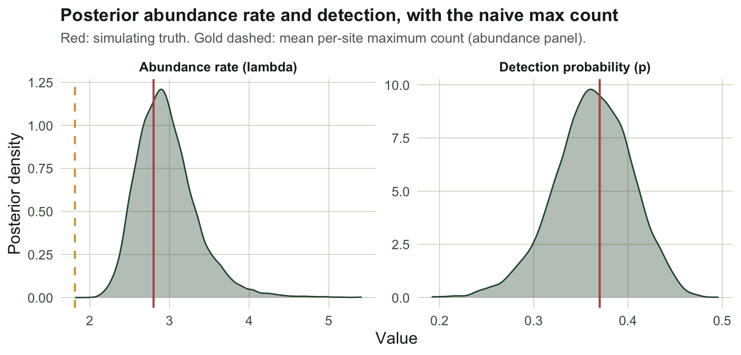
The total the maximum count throws away
Summing the latent counts in each draw gives a posterior for total abundance across all sites. It sits where the truth is, and well above the naive total.
sage <- "#93a87f"; paper <- "#f5f4ee"
ggplot(data.frame(value = Ntot.post), aes(value)) +
  geom_histogram(aes(y = after_stat(density)), bins = 45, fill = sage, colour = paper, linewidth = 0.15) +
  geom_vline(xintercept = true.total, colour = rust, linewidth = 0.8) +
  geom_vline(xintercept = naive.total, colour = gold, linewidth = 0.8, linetype = "dashed") +
  labs(title = "Posterior total abundance across all sites",
       subtitle = "Red: true total. Gold dashed: naive total from summed maximum counts.",
       x = "Total individuals", y = "Posterior density") + theme_te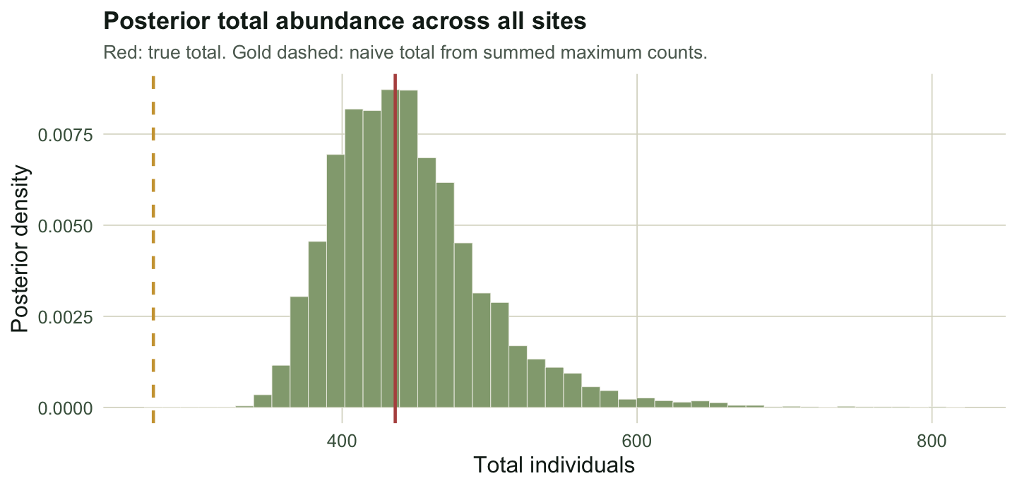
A caution on identifiability
The model leans hard on the between-visit variation, and with sparse data or few visits the abundance and detection parameters trade off: many animals seen rarely can mimic few animals seen often. Here 150 sites and four visits pin both down, but the N-mixture literature documents unstable estimates and infinite-abundance modes when the counts are thin, so check that the posterior is well behaved rather than assuming it. The latent-state sweep also induces autocorrelation, so run long and watch the effective sample size.
The pattern is the same one behind the Bayesian occupancy model, where the latent state is presence rather than a count, and the Bayesian survival model, where it is the alive-or-dead status of a marked animal. Put the unobserved quantity in the sampler and the awkward marginalisation disappears.
References
- Royle 2004, Biometrics 60(1):108-115 (10.1111/j.0006-341X.2004.00142.x)
- Barker, Schofield, Link, Sauer 2018, Biometrics 74(1):369-377 (10.1111/biom.12734)
- Kery 2018, Ecology 99(2):281-288 (10.1002/ecy.2093)
- Tanner, Wong 1987, Journal of the American Statistical Association 82(398):528-540 (10.1080/01621459.1987.10478458)
- Kery, Royle 2016, Applied Hierarchical Modeling in Ecology, ISBN 978-0-12-801378-6