---
title: "Bayesian model comparison: WAIC, LOO, DIC"
description: "Comparing Bayesian models for ecological count data in base R: coding WAIC, PSIS-LOO with the Pareto-k check and DIC from posterior draws, from scratch."
date: "2026-07-15 09:00"
categories: [R, Bayesian statistics, MCMC, model selection, ecology tutorial]
image: thumbnail.png
image-alt: "Four model-comparison scores across candidate models; in-sample deviance keeps dropping while WAIC, LOO and DIC bottom out at the true quadratic model."
---
```{r}
#| label: setup
#| include: false
knitr::opts_chunk$set(message = FALSE, warning = FALSE,
fig.width = 7.5, fig.height = 5.4, dpi = 150)
library(ggplot2)
te <- list(ink="#16241d", body="#2c3a31", forest="#275139", label="#46604a",
sage="#93a87f", paper="#f5f4ee", line="#dad9ca", faint="#5d6b61",
gold="#cda23f", mown="#2f8f63", terra="#b5534e")
theme_te <- function(base_size = 13) {
theme_minimal(base_size = base_size) +
theme(plot.background = element_rect(fill = te$paper, colour = NA),
panel.background = element_rect(fill = te$paper, colour = NA),
panel.grid.major = element_line(colour = te$line, linewidth = 0.3),
panel.grid.minor = element_blank(),
axis.text = element_text(colour = te$faint),
axis.title = element_text(colour = te$body),
plot.title = element_text(colour = te$ink, face = "bold"),
plot.subtitle = element_text(colour = te$label),
legend.text = element_text(colour = te$body),
plot.caption = element_text(colour = te$faint, size = base_size * 0.75))
}
```
A single fitted model tells you what it thinks; a set of fitted models makes you
choose. The trouble is that the obvious score, the fit to the data you already
have, always rewards the more complicated model. Add a parameter and the
likelihood can only go up, so the in-sample deviance points you at the most
flexible candidate every time, whether or not that flexibility describes anything
real.
The frequentist answer is to add a penalty to the maximised fit; that is what
[AIC does](../model-selection-aic/), using a single point estimate of the
parameters. The Bayesian versions use the whole posterior instead of a point:
the deviance information criterion (DIC), the widely applicable information
criterion (WAIC), and leave-one-out cross-validation approximated by
Pareto-smoothed importance sampling (PSIS-LOO). This post codes all three by hand
from posterior draws, on a small ecological count problem, and shows why the
in-sample number is not a model-selection tool at all.
## A hump-shaped count response
Abundance often peaks at an intermediate value of some gradient and falls away at
both ends, which a quadratic term on the log scale captures. We simulate counts
from exactly that structure and then pretend we do not know it.
```{r}
#| label: sim
set.seed(0)
n      <- 80
b_true <- c(1.0, 0.8, -0.7)                 # intercept, linear, quadratic
xsim   <- sort(runif(n, -2.2, 2.2))
Xfull  <- cbind(1, xsim, xsim^2)
y      <- rpois(n, exp(as.vector(Xfull %*% b_true)))
c(n = n, mean_count = round(mean(y), 2), zeros = sum(y == 0), max = max(y))
```
The candidates are nested: intercept only (`M0`), linear (`M1`), the true
quadratic (`M2`), and a cubic model (`M3`) that has one parameter too many.
## Fitting each model by MCMC
Every criterion below needs posterior draws, so we sample each model with a
random-walk [Metropolis sampler](../metropolis-hastings-from-scratch/). The
log-posterior is a Poisson log-likelihood plus a weakly-informative `N(0, 5^2)`
prior on each coefficient. The only shortcut is the proposal: we shape it with the
inverse Hessian at the maximum, scaled by the standard `2.4^2 / d` factor, so the
chain mixes without hand-tuning. The Metropolis step itself is coded out in full.
```{r}
#| label: mcmc
loglik_vec <- function(beta, X) dpois(y, exp(as.vector(X %*% beta)), log = TRUE)
logpost <- function(beta, X, ps = 5) {
  lam <- exp(as.vector(X %*% beta))
  if (any(!is.finite(lam)) || any(lam > 1e8)) return(-Inf)
  sum(dpois(y, lam, log = TRUE)) + sum(dnorm(beta, 0, ps, log = TRUE))
}
run_mcmc <- function(X, iter = 30000, warm = 5000, seed = 1) {
  set.seed(seed)
  d   <- ncol(X)
  fit <- optim(rep(0, d), function(b) -logpost(b, X), method = "BFGS", hessian = TRUE)
  Cp  <- chol(solve(fit$hessian) * (2.4^2 / d))     # proposal Cholesky
  beta <- fit$par; lp <- logpost(beta, X)
  out <- matrix(NA_real_, iter, d); acc <- 0
  for (t in seq_len(iter)) {
    prop <- beta + as.vector(crossprod(Cp, rnorm(d)))
    lpp  <- logpost(prop, X)
    if (log(runif(1)) < lpp - lp) { beta <- prop; lp <- lpp; acc <- acc + 1 }
    out[t, ] <- beta
  }
  draws <- out[(warm + 1):iter, , drop = FALSE]
  ll <- matrix(NA_real_, nrow(draws), length(y))       # S x n log-likelihood
  for (s in seq_len(nrow(draws))) ll[s, ] <- loglik_vec(draws[s, ], X)
  list(draws = draws, ll = ll, acc = acc / iter)
}

Xlist <- list(M0 = Xfull[, 1, drop = FALSE], M1 = Xfull[, 1:2],
              M2 = Xfull[, 1:3], M3 = cbind(Xfull, xsim^3))
fits  <- Map(function(X, s) run_mcmc(X, seed = s), Xlist, c(101, 202, 303, 404))
```
The pointwise log-likelihood matrix `ll`, with one row per draw and one column per
observation, is the single object all three criteria are built from. The
acceptance rates sit near the random-walk optimum
(`r paste(sprintf("%.2f", sapply(fits, function(f) f$acc)), collapse = ", ")` for
`M0` to `M3`), and the quadratic model recovers the truth: its posterior mean is
`r paste(sprintf("%.3f", colMeans(fits$M2$draws)), collapse = ", ")` against the
generating `r paste(b_true, collapse = ", ")`.
## The naive number: in-sample deviance
The deviance at the maximum, `-2` times the maximised log-likelihood, is the fit
component that AIC starts from. Because the models are nested, it can only fall as
parameters are added.
```{r}
#| label: naive
naive_dev <- sapply(Xlist, function(X) {
  Xm <- X; -2 * as.numeric(logLik(glm(y ~ Xm - 1, family = poisson)))
})
round(naive_dev, 1)
```
The linear-to-quadratic drop is real: leaving out the curvature costs a great
deal. But the quadratic-to-cubic step does not move at all
(`r round(naive_dev["M2"], 1)` for both `M2` and `M3`): the extra parameter buys
nothing here, yet the in-sample rule is at best indifferent between them and would
pick whichever is lower by chance. It never charges you for the flexibility. That
is the whole problem, and every criterion below is a way of estimating the price.
## DIC
DIC uses the posterior distribution of the deviance. Let `Dbar` be the posterior
mean of `-2` log-likelihood and let `D(thetabar)` be the deviance at the posterior
mean of the parameters. The effective number of parameters is their difference,
`pD = Dbar - D(thetabar)`, and `DIC = Dbar + pD` (Spiegelhalter 2002).
```{r}
#| label: dic
dic_one <- function(m, X) {
  Dbar <- mean(-2 * rowSums(m$ll))
  Dhat <- -2 * sum(loglik_vec(colMeans(m$draws), X))
  pD <- Dbar - Dhat
  c(DIC = Dbar + pD, pD = pD)
}
```
## WAIC
WAIC works observation by observation and never touches a point estimate. The log
pointwise predictive density averages the likelihood over the posterior at each
point, `lppd_i = log mean_s p(y_i | theta_s)`; the effective parameter count is the
posterior variance of the log-likelihood at each point,
`pWAIC_i = var_s log p(y_i | theta_s)`. Then
`WAIC = -2 (sum_i lppd_i - sum_i pWAIC_i)` (Watanabe's criterion in the Bayesian
framing of Gelman 2014).
```{r}
#| label: waic
waic_one <- function(m) {
  cm  <- apply(m$ll, 2, max)                             # log-sum-exp, stably
  lppd <- cm + log(colMeans(exp(sweep(m$ll, 2, cm))))
  pw   <- apply(m$ll, 2, var)
  list(WAIC = -2 * sum(lppd - pw), pWAIC = sum(pw),
       pt = lppd - pw)                                   # pointwise elpd
}
```
## PSIS-LOO and the Pareto-k check
Leave-one-out cross-validation asks how well the model predicts each point when
that point is held out. Refitting `n` times is expensive, but the held-out
predictive density can be estimated from the single full-data fit by importance
sampling: the weight for draw `s` at point `i` is `1 / p(y_i | theta_s)`. Those raw
weights have heavy tails and occasionally one draw dominates, which is where
PSIS-LOO improves on plain importance sampling (Vehtari 2017): it fits a
generalised Pareto distribution to the largest weights and replaces them with the
fitted quantiles. The estimated Pareto shape, `k-hat`, is also a diagnostic:
`k > 0.7` means the importance-sampling estimate for that point is not to be
trusted.
The Pareto fit uses the empirical-Bayes estimator of Zhang and Stephens (2009),
coded here in full.
```{r}
#| label: gpd
gpdfit <- function(x) {                       # x: exceedances, ascending, > 0
  N <- length(x); m <- 30 + floor(sqrt(N))
  bs <- 1 - sqrt(m / (seq_len(m) - 0.5))
  bs <- bs / (3 * x[floor(N / 4 + 0.5)]) + 1 / x[N]
  ks <- vapply(bs, function(b) mean(log1p(-b * x)), numeric(1))
  L  <- N * (log(-bs / ks) - ks - 1)
  w  <- 1 / vapply(seq_len(m), function(j) sum(exp(L - L[j])), numeric(1))
  b  <- sum(bs * w); k <- mean(log1p(-b * x))
  list(k = (k * N + 5) / (N + 10), sigma = -k / b)       # prior-shrunk k, scale
}
qgpd <- function(p, k, sig)
  if (abs(k) < 1e-9) -sig * log1p(-p) else sig / k * ((1 - p)^(-k) - 1)

psis_i <- function(logr) {                    # log importance ratios, one point
  S <- length(logr); r <- exp(logr - max(logr))
  M <- ceiling(min(0.2 * S, 3 * sqrt(S)))
  ord <- order(r); u <- r[ord][S - M]; tail_i <- ord[(S - M + 1):S]
  g <- gpdfit(r[tail_i] - u)
  r[tail_i] <- pmin(u + qgpd((seq_len(M) - 0.5) / M, g$k, g$sigma), max(r))
  list(w = r / sum(r), k = g$k)
}

loo_one <- function(m) {
  nn <- ncol(m$ll); ei <- numeric(nn); kh <- numeric(nn)
  for (i in seq_len(nn)) {
    ps <- psis_i(-m$ll[, i])                             # ratios 1 / p_i
    a  <- m$ll[, i]; mx <- max(a)
    ei[i] <- mx + log(sum(ps$w * exp(a - mx)))           # weighted predictive
    kh[i] <- ps$k
  }
  list(LOO = -2 * sum(ei), elpd = ei, khat = kh)
}
```
## Putting the scores side by side
```{r}
#| label: table
ics <- lapply(names(Xlist), function(nm) {
  m <- fits[[nm]]; X <- Xlist[[nm]]
  d <- dic_one(m, X); w <- waic_one(m); l <- loo_one(m)
  list(in_sample = naive_dev[[nm]], DIC = d["DIC"], pD = d["pD"],
       WAIC = w$WAIC, pWAIC = w$pWAIC, pt = w$pt,
       LOO = l$LOO, khat = l$khat, p_loo = w$pWAIC)
})
names(ics) <- names(Xlist)
aic <- sapply(Xlist, function(X) { Xm <- X; AIC(glm(y ~ Xm - 1, family = poisson)) })

tab <- data.frame(
  model = names(Xlist), parameters = sapply(Xlist, ncol),
  in_sample = round(naive_dev, 1),
  DIC = round(sapply(ics, `[[`, "DIC"), 1), pD = round(sapply(ics, `[[`, "pD"), 2),
  WAIC = round(sapply(ics, `[[`, "WAIC"), 1),
  pWAIC = round(sapply(ics, `[[`, "pWAIC"), 2),
  LOO = round(sapply(ics, `[[`, "LOO"), 1), AIC = round(aic, 1),
  max_k = round(sapply(ics, function(z) max(z$khat)), 2), row.names = NULL)
tab
```
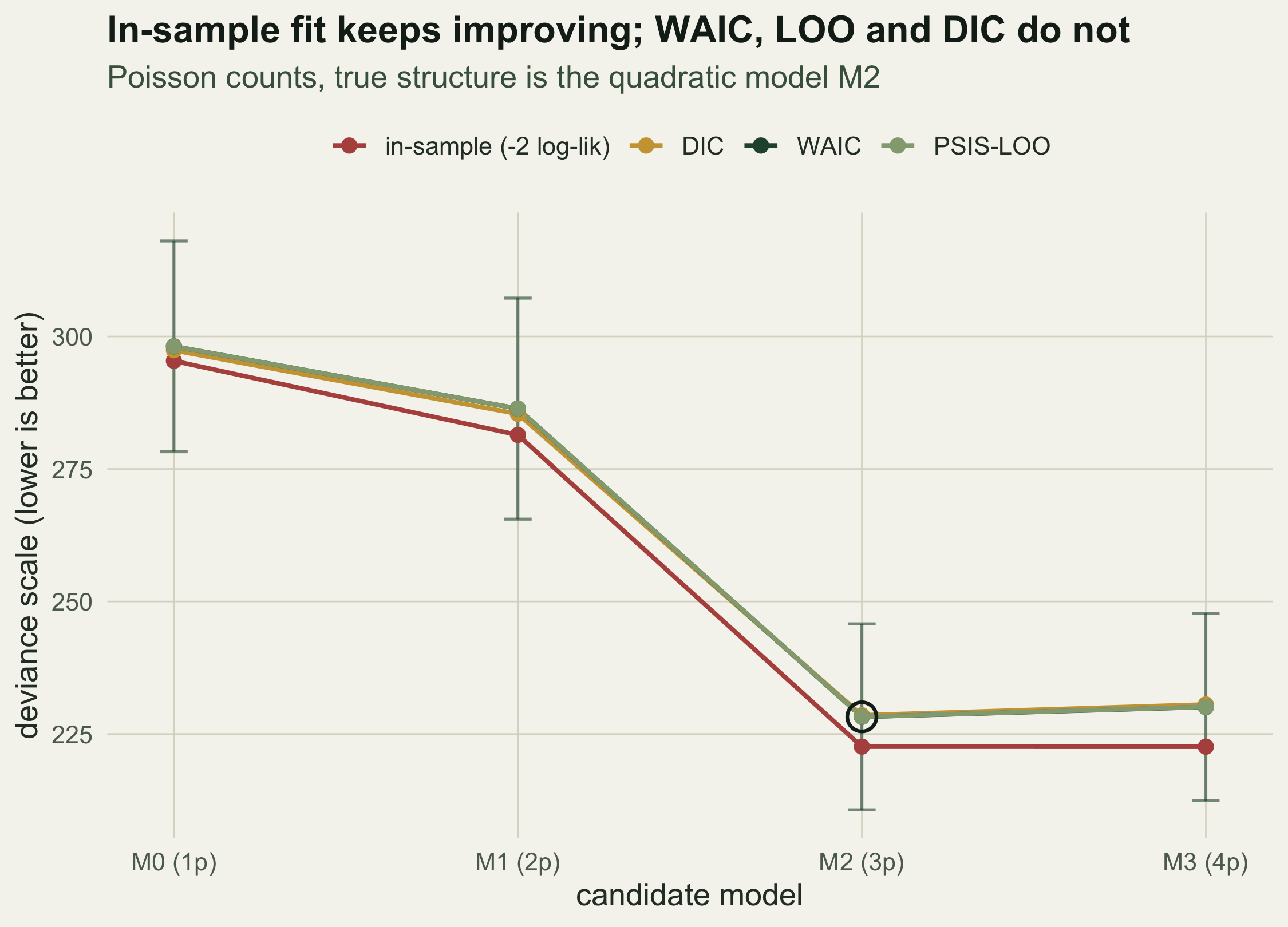
Every criterion that estimates out-of-sample loss agrees, and disagrees with the
in-sample number. In-sample deviance is flat across the last step; DIC, WAIC,
PSIS-LOO and AIC all put the minimum at the true quadratic model and charge the
cubic model roughly two deviance units for its spare parameter. The effective
parameter counts (`pWAIC` and `pD`) track the actual dimensions, and no Pareto
`k-hat` exceeds `r round(max(sapply(ics, function(z) max(z$khat))), 2)`, so the
importance sampling is stable throughout.
```{r}
#| label: fig-scores
#| fig-cap: "In-sample deviance falls or flattens as parameters are added, so it never prefers the true model M2 over the larger M3. DIC, WAIC and PSIS-LOO estimate out-of-sample loss and share a minimum at M2; the error bars are the WAIC standard error."
#| fig-alt: "Line plot of deviance-scale scores against the four candidate models M0 to M3. The in-sample line falls steeply then stays flat from M2 to M3. The DIC, WAIC and PSIS-LOO lines all reach their lowest value at M2 and rise slightly at M3, with the M2 WAIC point ringed."
np  <- sapply(Xlist, ncol)
seW <- sapply(names(Xlist), function(nm) 2 * sqrt(n * var(ics[[nm]]$pt)))
mk  <- function(v, lab) data.frame(npar = np, score = v, kind = lab)
df1 <- rbind(mk(naive_dev, "in-sample (-2 log-lik)"), mk(sapply(ics, `[[`, "DIC"), "DIC"),
             mk(sapply(ics, `[[`, "WAIC"), "WAIC"), mk(sapply(ics, `[[`, "LOO"), "PSIS-LOO"))
df1$kind <- factor(df1$kind, levels = c("in-sample (-2 log-lik)", "DIC", "WAIC", "PSIS-LOO"))
best <- which.min(sapply(ics, `[[`, "WAIC"))
dfW <- data.frame(npar = np, WAIC = sapply(ics, `[[`, "WAIC"), se = seW)
ggplot(df1, aes(npar, score, colour = kind)) +
  geom_errorbar(data = dfW, inherit.aes = FALSE,
                aes(npar, ymin = WAIC - se, ymax = WAIC + se), width = 0.08,
                colour = te$forest, alpha = 0.6) +
  geom_line(linewidth = 0.9) + geom_point(size = 2.4) +
  annotate("point", x = np[best], y = sapply(ics, `[[`, "WAIC")[best],
           size = 5, shape = 21, stroke = 1.1, colour = te$ink, fill = NA) +
  scale_colour_manual(values = c("in-sample (-2 log-lik)" = te$terra, "DIC" = te$gold,
                                 "WAIC" = te$forest, "PSIS-LOO" = te$sage), name = NULL) +
  scale_x_continuous(breaks = np, labels = paste0(names(Xlist), " (", np, "p)")) +
  labs(x = "candidate model", y = "deviance scale (lower is better)",
       title = "In-sample fit keeps improving; WAIC, LOO and DIC do not",
       subtitle = "Poisson counts, true structure is the quadratic model M2") +
  theme_te() + theme(legend.position = "top")
```
The size of a difference matters as much as its sign, and PSIS-LOO carries a
standard error for it. The gap between the quadratic and the cubic model is small
but real (an elpd difference of
`r sprintf("%.2f", { d <- ics$M2$pt - ics$M3$pt; sum(d) })` with a standard error
of `r sprintf("%.2f", { d <- ics$M2$pt - ics$M3$pt; sqrt(n * var(d)) })`), so we
prefer the simpler true model without pretending the cubic is badly wrong.
Dropping to the linear model is a different matter: that difference is
`r sprintf("%.1f", { d <- ics$M2$pt - ics$M1$pt; sum(d) })` with a standard error
of `r sprintf("%.1f", { d <- ics$M2$pt - ics$M1$pt; sqrt(n * var(d)) })`, decisive
by any reading.
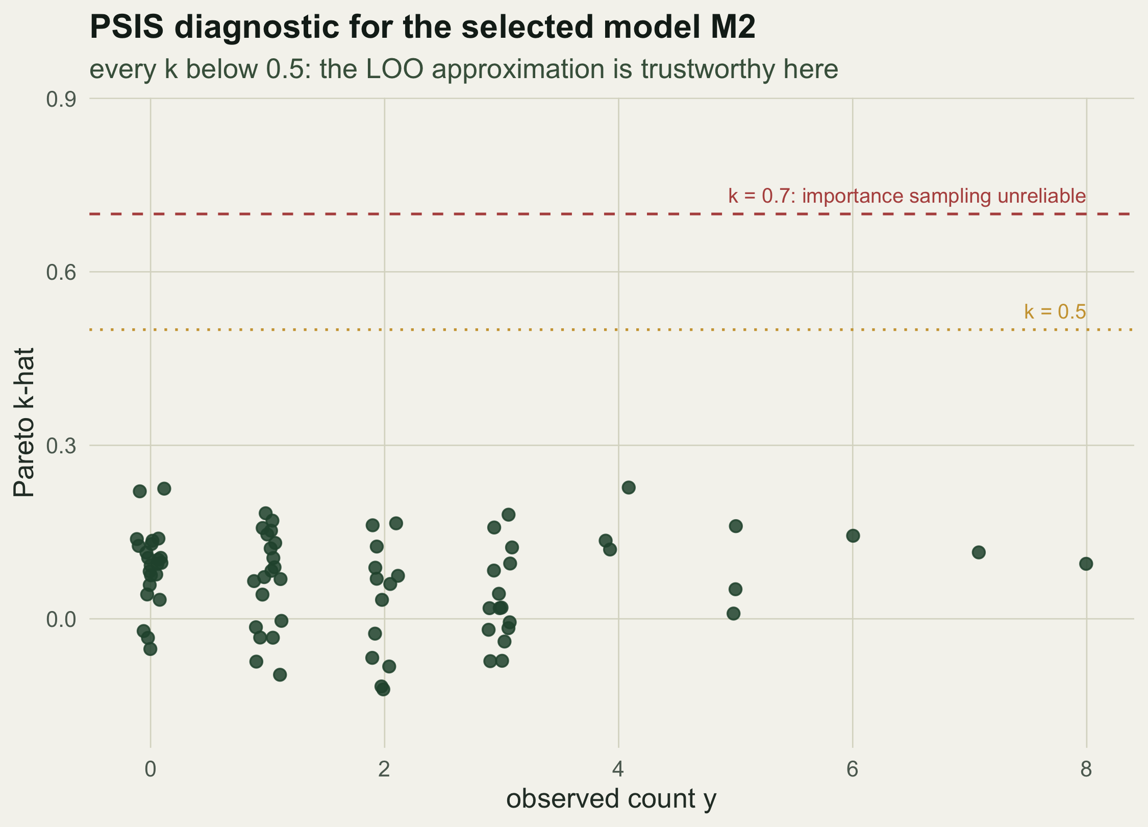
## Reading the Pareto-k diagnostic
The `k-hat` values are worth plotting in their own right, because they tell you
when the LOO number can be believed. Here they climb gently with the size of the
count, which is expected: a large observation pulls harder on the fit and is
therefore closer to being influential. None of them crosses even the cautionary
`0.5` line.
```{r}
#| label: fig-pareto
#| fig-cap: "Pareto k-hat for each observation under the selected model M2. All values sit below 0.5, so the PSIS-LOO estimate is reliable for every point; k above 0.7 would flag observations where the importance-sampling approximation fails and exact leave-one-out is needed."
#| fig-alt: "Scatter of Pareto k-hat against observed count for the quadratic model. Points rise gently from about 0.05 to 0.25 as the count grows, all well below the dotted 0.5 line and the dashed 0.7 threshold."
kk <- ics[[best]]$khat
ggplot(data.frame(y = y, k = kk), aes(y, k)) +
  geom_hline(yintercept = 0.7, linetype = "dashed", colour = te$terra) +
  geom_hline(yintercept = 0.5, linetype = "dotted", colour = te$gold) +
  geom_jitter(width = 0.12, height = 0, size = 2.3, colour = te$forest, alpha = 0.85) +
  annotate("text", x = max(y), y = 0.72, hjust = 1, vjust = 0, size = 3.4,
           colour = te$terra, label = "k = 0.7: importance sampling unreliable") +
  annotate("text", x = max(y), y = 0.52, hjust = 1, vjust = 0, size = 3.4,
           colour = te$gold, label = "k = 0.5") +
  coord_cartesian(ylim = c(min(kk) - 0.05, 0.85)) +
  labs(x = "observed count y", y = "Pareto k-hat",
       title = "PSIS diagnostic for the selected model M2",
       subtitle = "every k below 0.5: the LOO approximation is trustworthy here") +
  theme_te()
```
## Which one to reach for
For most models fitted by MCMC, PSIS-LOO is the one to report: it estimates the
same predictive quantity as WAIC but degrades more gracefully with weak priors or
influential points, and its `k-hat` values tell you exactly where it is failing.
WAIC is a cheaper approximation to the same target and agrees with LOO here, as it
should in a well-behaved problem. DIC is the oldest of the three and the least
safe, because it collapses the posterior to a single point through `D(thetabar)`;
in mixture or weakly-identified models that plug-in can misbehave, and `pD` can
even go negative. All three rest on splitting the data into the units you want to
predict, which for these independent counts is one observation each; for grouped
or time-structured data the unit is a decision in itself, not a default.
The deeper point is the one the in-sample column makes for free. Fit to the data
in hand is not evidence about a model, because it cannot see the cost of
flexibility. Only an estimate of out-of-sample loss can, and the Bayesian versions
build that estimate out of the same posterior draws you already have.
## References
- Akaike H 1974 IEEE Transactions on Automatic Control 19(6):716-723 (10.1109/TAC.1974.1100705)
- Spiegelhalter DJ, Best NG, Carlin BP, van der Linde A 2002 Journal of the Royal Statistical Society B 64(4):583-639 (10.1111/1467-9868.00353)
- Gelman A, Hwang J, Vehtari A 2014 Statistics and Computing 24(6):997-1016 (10.1007/s11222-013-9416-2)
- Vehtari A, Gelman A, Gabry J 2017 Statistics and Computing 27(5):1413-1432 (10.1007/s11222-016-9696-4)
- Zhang J, Stephens MA 2009 Technometrics 51(3):316-325 (10.1198/tech.2009.08017)
- Gelman A, Carlin JB, Stern HS, Dunson DB, Vehtari A, Rubin DB 2013 Bayesian Data Analysis, 3rd edn (ISBN 978-1-4398-4095-5)
- McElreath R 2020 Statistical Rethinking, 2nd edn (ISBN 978-0-367-13991-9)
## Related tutorials
- [Model selection with AIC, AICc and BIC](../model-selection-aic/)
- [Metropolis-Hastings from scratch](../metropolis-hastings-from-scratch/)
- [MCMC convergence diagnostics from scratch](../mcmc-convergence-diagnostics/)
- [Modelling count data with GLMs](../glm-count-data-abundance/)