Checking a reputation model

Three diagnostics for indirect reciprocity models in R: sensitivity to the benefit-to-cost ratio, replication across seeds, and drift in a finite population.

The three previous posts produced tidy results: a threshold at q > c/b, a clean split between assessment rules, and a reversal of that split under private information. Every one of those rests on choices that were never tested. The benefit and cost were fixed at 3 and 1. The agent-based runs used a single seed. Selection was treated as deterministic, in populations that are actually finite. This post runs the three checks that those choices invite, and one of the earlier results does not come through intact.

Check 1: does the threshold depend on the payoffs?

The threshold q > c/b was derived with b = 3 and c = 1, giving one third. The ratio is the only thing that enters, so the check is quick and the answer is reassuring in form but not in magnitude.

for (ratio in c(1.5, 2, 3, 5, 10))
  cat(sprintf("b/c = %4.1f   reputation must be known more than %.2f of the time\n",
              ratio, 1 / ratio))

b/c =  1.5   reputation must be known more than 0.67 of the time
b/c =  2.0   reputation must be known more than 0.50 of the time
b/c =  3.0   reputation must be known more than 0.33 of the time
b/c =  5.0   reputation must be known more than 0.20 of the time
b/c = 10.0   reputation must be known more than 0.10 of the time

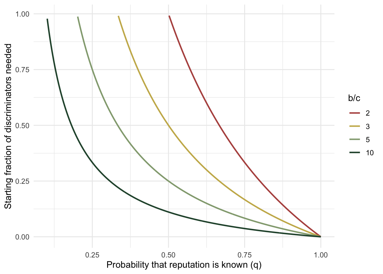
The structure survives any ratio: there is always a threshold, and it always falls as helping gets cheaper relative to its benefit. What moves is how demanding the condition is. At a ratio of 2 a donor must know its recipient’s record in more than half of all encounters, which is a strong requirement outside small groups. At a ratio of 10 one encounter in ten is enough.

That matters for interpreting field systems. Reporting that a species has a plausible b/c ratio says nothing on its own; the same ratio implies a demanding information requirement in one case and a lax one in another, and the information side is the harder one to measure.

The separatrix moves in the same direction, and more steeply.

library(ggplot2)
sep <- function(q, ratio) (1 - q) / (q * (ratio - 1))       # x* with c = 1, b = ratio
d <- do.call(rbind, lapply(c(2, 3, 5, 10), function(ratio) {
  q <- seq(1 / ratio + 0.002, 1, 0.002)
  data.frame(q = q, x = sep(q, ratio), ratio = factor(ratio))
}))
d <- d[d$x <= 1, ]
ggplot(d, aes(q, x, colour = ratio)) +
  geom_line(linewidth = 0.9) +
  scale_colour_manual(values = c("2" = "#b5534e", "3" = "#c9b458",
                                 "5" = "#93a87f", "10" = "#275139")) +
  labs(x = "Probability that reputation is known (q)",
       y = "Starting fraction of discriminators needed", colour = "b/c") +
  theme_minimal(base_size = 12)

Figure 1: The starting fraction of discriminators needed for cooperation to take over, for four benefit-to-cost ratios. Each curve leaves the unit interval below its own threshold q = c/b.

Check 2: is the private-information result one lucky seed?

The private-information model was run once per cell with the seed fixed at 449. A single run of an agent-based model is a single draw, and reporting it to three decimals implies a precision it has not earned. Repeat each rule across ten seeds at q = 0.5 and look at the spread.

run <- function(q, rule, N = 100, rounds = 400, e = 0.02, seed = 1) {
  set.seed(seed)
  opinion <- matrix(1L, N, N)
  coop <- numeric(rounds)
  for (r in seq_len(rounds)) {
    ord <- sample.int(N)
    donors <- ord[1:(N / 2)]; recips <- ord[(N / 2 + 1):N]
    helped <- 0
    for (k in seq_along(donors)) {
      d <- donors[k]; v <- recips[k]
      act <- opinion[d, v] == 1L && runif(1) > e
      helped <- helped + act
      obs <- union(which(runif(N) < q), d)
      rec_good <- opinion[cbind(obs, v)] == 1L
      opinion[cbind(obs, d)] <- switch(rule,
        standing = as.integer(act | !rec_good),
        stern    = as.integer(ifelse(rec_good, act, !act)),
        scoring  = as.integer(rep(act, length(obs))))
    }
    coop[r] <- helped / length(donors)
  }
  mean(tail(coop, 100))
}

seeds <- 1:10
reps <- sapply(c("standing", "stern", "scoring"),
               function(rule) sapply(seeds, function(s) run(0.5, rule, seed = s)))
round(rbind(mean = colMeans(reps), sd = apply(reps, 2, sd),
            min = apply(reps, 2, min), max = apply(reps, 2, max)), 3)

     standing stern scoring
mean    0.918 0.490   0.176
sd      0.012 0.007   0.168
min     0.898 0.476   0.003
max     0.936 0.496   0.415

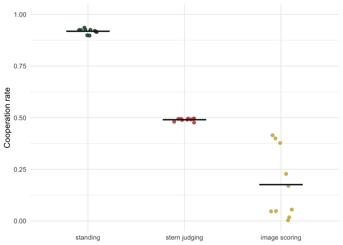
Two of the three rules are solid. Standing gives 0.918 with a standard deviation of 0.012, stern judging 0.490 with 0.007. Neither ranking would change under any seed, and the collapse of stern judging to roughly half is a real feature of the rule rather than an artefact.

Image scoring is a different matter. Its mean of 0.176 comes with a standard deviation of 0.168 and a range from 0.003 to 0.415: some seeds produce almost no cooperation, others more than 40 per cent. The claim in the previous post that image scoring improves under private information is therefore much weaker than it looked. The direction is right on average, but a single run tells you almost nothing, and any statement about the size of the effect needs the spread attached.

long <- data.frame(rule = rep(c("standing", "stern judging", "image scoring"), each = length(seeds)),
                   cooperation = as.vector(reps))
long$rule <- factor(long$rule, levels = c("standing", "stern judging", "image scoring"))
ggplot(long, aes(rule, cooperation, colour = rule)) +
  geom_jitter(width = 0.12, height = 0, size = 2, alpha = 0.85) +
  stat_summary(fun = mean, geom = "crossbar", width = 0.45, linewidth = 0.4, colour = "#16241d") +
  scale_colour_manual(values = c(standing = "#275139", `stern judging` = "#b5534e",
                                 `image scoring` = "#c9b458"), guide = "none") +
  coord_cartesian(ylim = c(0, 1)) +
  labs(x = NULL, y = "Cooperation rate") +
  theme_minimal(base_size = 12)

Figure 2: Cooperation at q = 0.5 across ten random seeds. Standing and stern judging are tightly clustered; image scoring scatters across the whole range, so its single-seed value carries little information.

Check 3: is the free rider really removed?

The assessment rules post reported that discriminators out-earn unconditional helpers by 0.0452 under standing and 0.1773 under stern judging, and treated both as selection against the second-order free rider. In an infinite population that is fair. In a finite one, a disadvantage that small competes with drift, and the right question is not the sign of the gap but the probability that the free rider takes over anyway.

The Moran process gives that probability directly. For a mutant with fitness ratio r in a population of N, the chance it reaches fixation is (1 - 1/r) / (1 - 1/r^N), which reduces to 1/N when r is one.

b <- 3; cost <- 1
rules <- list(standing = matrix(c(1, 1, 0, 1), 2, 2),
              `stern judging` = matrix(c(1, 0, 0, 1), 2, 2))
strategies <- list(DISC = c(1, 0), ALLC = c(1, 1))

payoffs <- function(rule, mix, e = 0.05, iters = 2000) {
  A <- rules[[rule]]; nm <- names(mix)
  g <- setNames(rep(1, length(mix)), nm)
  for (it in seq_len(iters)) {
    gbar <- sum(mix * g); prior <- c(gbar, 1 - gbar)
    g_new <- sapply(nm, function(i) {
      p <- strategies[[i]] * (1 - e); sum(prior * (p * A[, 1] + (1 - p) * A[, 2])) })
    if (max(abs(g_new - g)) < 1e-12) { g <- g_new; break }
    g <- g_new
  }
  gbar <- sum(mix * g)
  helping <- sapply(nm, function(i) sum(c(gbar, 1 - gbar) * strategies[[i]] * (1 - e)))
  received <- sapply(nm, function(i) sum(sapply(nm, function(j)
    mix[j] * (1 - e) * (g[i] * strategies[[j]][1] + (1 - g[i]) * strategies[[j]][2]))))
  -cost * helping + b * received
}

fixation <- function(r, N = 100) if (abs(r - 1) < 1e-12) 1 / N else (1 - 1 / r) / (1 - 1 / r^N)

for (rule in names(rules)) {
  p <- payoffs(rule, c(DISC = 0.90, ALLC = 0.10))
  rel <- p["ALLC"] / p["DISC"]
  cat(sprintf("%-14s gap %+0.4f  relative fitness %.4f  fixation %.5f  (neutral %.5f)\n",
              rule, p["DISC"] - p["ALLC"], rel, fixation(rel), 0.01))
}

standing       gap +0.0452  relative fitness 0.9752  fixation 0.00224  (neutral 0.01000)
stern judging  gap +0.1773  relative fitness 0.9030  fixation 0.00000  (neutral 0.01000)

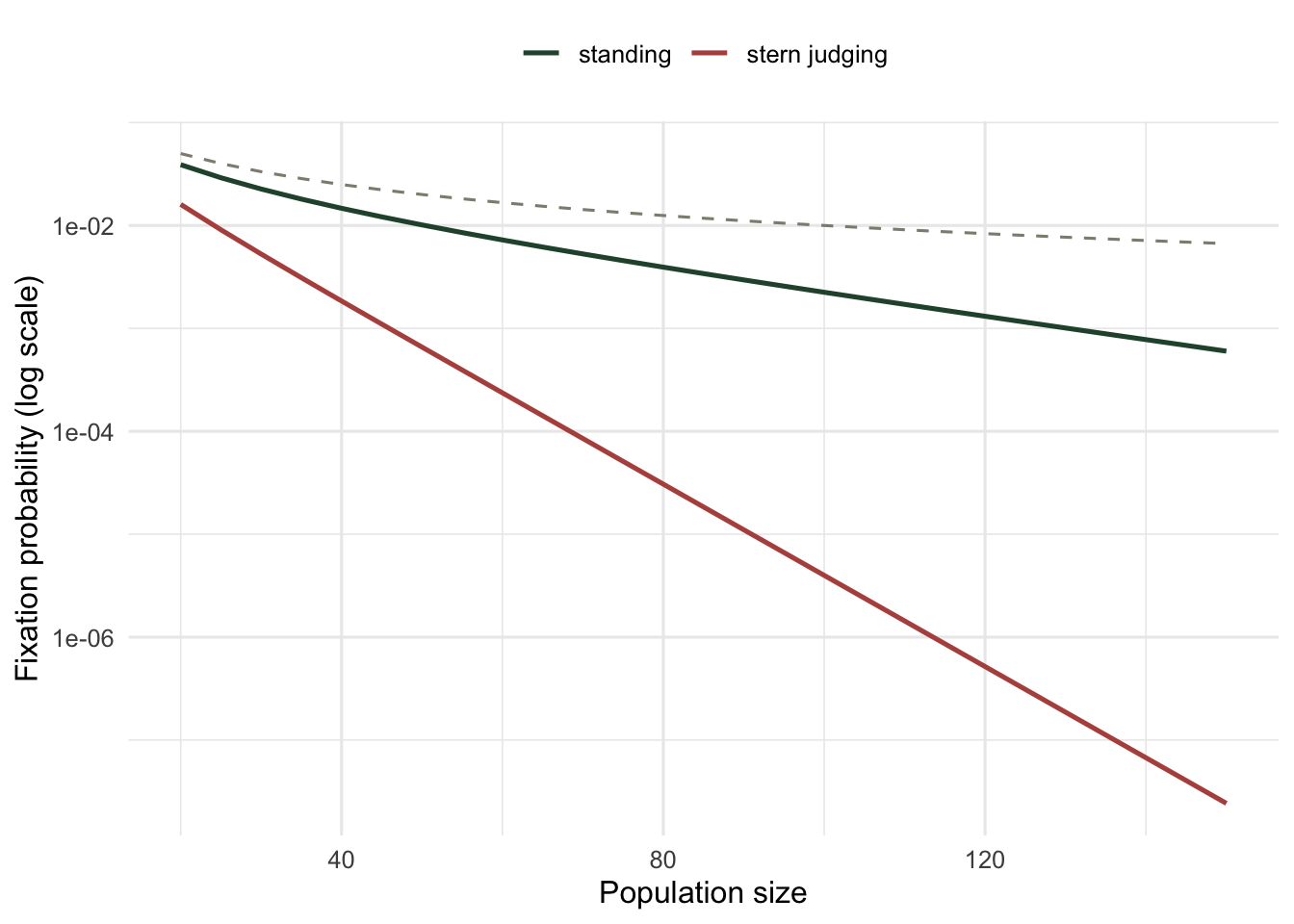
Under standing the free rider’s relative fitness is 0.9752, giving a fixation probability of 0.00224 against the neutral 0.01. Selection is working, but it is only about four and a half times stronger than drift, so in a population of a hundred an unconditional helper still takes over roughly once in every 450 introductions. Under stern judging relative fitness is 0.9030 and fixation rounds to zero at five decimal places, which is a different regime entirely.

The size of the population decides how much of this matters.

Ns <- seq(20, 150, 5)
rel <- sapply(names(rules), function(rule) {
  p <- payoffs(rule, c(DISC = 0.90, ALLC = 0.10)); as.numeric(p["ALLC"] / p["DISC"]) })
fx <- do.call(rbind, lapply(names(rules), function(rule)
  data.frame(N = Ns, p = sapply(Ns, function(n) fixation(rel[[rule]], n)), rule = rule)))
neutral <- data.frame(N = Ns, p = 1 / Ns)
ggplot(fx, aes(N, p, colour = rule)) +
  geom_line(data = neutral, aes(N, p), inherit.aes = FALSE,
            linetype = "dashed", colour = "#8d8d80") +
  geom_line(linewidth = 0.9) +
  scale_y_log10() +
  scale_colour_manual(values = c(standing = "#275139", `stern judging` = "#b5534e")) +
  labs(x = "Population size", y = "Fixation probability (log scale)", colour = NULL) +
  theme_minimal(base_size = 12) + theme(legend.position = "top")

Figure 3: Fixation probability of an unconditional helper introduced into a discriminating population, against population size. The dashed line is the neutral expectation 1/N; standing tracks it more closely than stern judging at every size.

In small groups the two rules are hard to tell apart, because drift swamps a fitness difference of a few per cent either way. The gap between them opens as the population grows. Any claim that stern judging is the stricter rule is therefore a claim about large populations, and the model should say so.

An honest limit

These checks probe the model’s own assumptions, not its correspondence to any animal. Nothing here tells you whether a species tracks third-party reputation at all, which is the question a field study would have to answer first, and the evidence for it outside humans and a few cleaner fish systems is thin.

The fitness ratios in check 3 also come from the deterministic equilibrium and are then dropped into a Moran process, which mixes an infinite-population calculation with a finite-population one. A fully finite model would let reputations fluctuate with the composition of the population, and the fixation probabilities would move. The direction of the comparison is safe; the fifth decimal is not.

Related tutorials

• Indirect reciprocity and reputation
• Assessment rules for reputation
• Public and private reputation
• Checking a reciprocity model

References

Nowak MA, Sasaki A, Taylor C, Fudenberg D 2004. Nature 428(6983):646-650 (10.1038/nature02414)

Ohtsuki H, Iwasa Y 2006. Journal of Theoretical Biology 239(4):435-444 (10.1016/j.jtbi.2005.08.008)

Hilbe C, Schmid L, Tkadlec J, Chatterjee K, Nowak MA 2018. Proceedings of the National Academy of Sciences 115(48):12241-12246 (10.1073/pnas.1810565115)